Advanced Objects
This chapter covers three objects designed to visualize mathematical fields: ContourPlot, which draws level curves of a scalar field; DensityPlot, which paints a scalar field as a colored raster; and VectorFieldPlot, which draws a planar vector field as a grid of arrows. All three share a common design: they sample a user-supplied function over a rectangular domain, they can be recolored with a ColorScale, and they implement the Parametric interface, so an extra t parameter in the function can be animated with play.scalar.
Table of Contents
The ContourPlot Class
The ContourPlot class generates level-curve (contour) shapes from a scalar field f(x, y) using the Marching Squares algorithm. It's a subclass of MultiShapeObject, so each contour line is an individual Shape child that can be styled, colored or animated independently.
Creating a ContourPlot
// f(x,y) = x^2 + y^2, domain is the current math view, 100x100 grid
def cp = ContourPlot.make(
    { x, y -> x * x + y * y },
    0.2, 0.7, 1.0            // level values c where f(x,y) = c
)

scene.add(cp)
You can also specify the domain and grid resolution explicitly:
def cp = ContourPlot.make(
    { x, y -> Math.sin(x) * Math.cos(y) },
    -1, 1, -1, 1,   // xMin, xMax, yMin, yMax
    150, 150,       // cols, rows
    -0.5, 0, 0.5    // levels
)

scene.add(cp)
Note: Levels don't need to be listed one by one. Any Collection<Number> is accepted too, for example a Groovy range like (-1..1).step(0.25).
Generating a Large Set of Levels
Typing out dozens of levels by hand doesn't scale. The Pythonizer class exposes a handful of Python/NumPy-style helpers (arange, linspace, ...) that are available directly in any script, without any prefix, so you can build the levels array programmatically:
// From -1 to 1 in steps of 0.1 (NumPy-style arange: stop is exclusive, so nudge it slightly)
def levels = arange(-1, 1 + 0.05, 0.1)

def cp = ContourPlot.make(
    { x, y -> Math.sin(x) * Math.sin(x) + Math.cos(x) * Math.cos(y) },
    -3, 3, -3, 3,
    150, 150,
    levels
)

scene.add(cp)
linspace is often more convenient when you know how many levels you want rather than the step size, since it always includes both endpoints:
// 21 evenly spaced levels between -1 and 1 (both endpoints included)
def levels = linspace(-1, 1, 21)

def cp = ContourPlot.make(
    { x, y -> Math.sin(x) * Math.sin(x) + Math.cos(x) * Math.cos(y) },
    -3, 3, -3, 3,
    150, 150,
    levels
)

scene.add(cp)
Note: arange(start, stop, step) mirrors NumPy: stop is exclusive, so to include an endpoint like 1.0 you need to push stop slightly past it (as in 1 + 0.05) to avoid losing it to floating-point rounding. linspace(start, stop, n) avoids this problem, since both endpoints are always included by design.
Coloring by Level
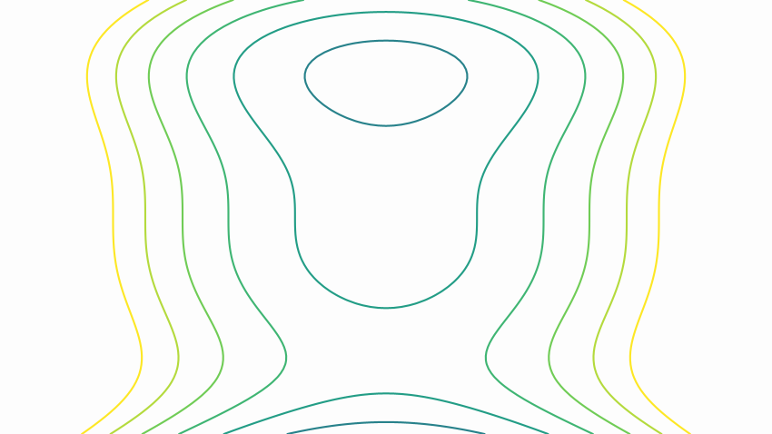
ContourPlot implements ColorScalable, so each contour can be colored according to its level value:
scene.add(Axes.make())
def cp = ContourPlot.make(
      {x, y -> x*x-y*y*Math.sin(PI*y)},
      linspace(-2, 2, 10))    // 10 numbers, from -2 to 2 (both included)
cp.applyColorScale(ColorScale.viridis(-2, 2)) //Creates viridis color scale for values from -2 to 2
scene.add(cp)
Animating the Field
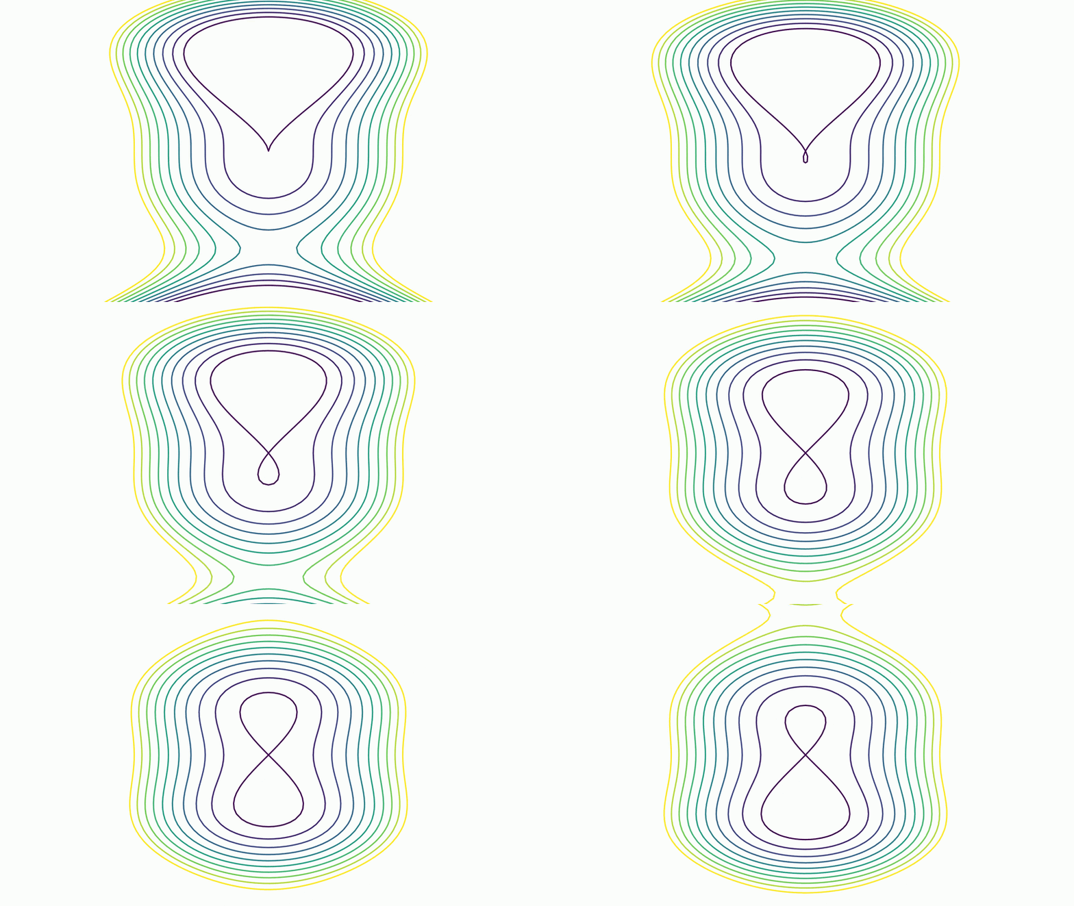
If the function takes a third parameter t, ContourPlot treats it as an animatable value exposed through getValue()/setValue(). This lets you animate it with play.scalar, which recomputes the contours on every frame:
def cp = ContourPlot.make(
     {x, y, t -> x*x-y*y*Math.sin(PI*y+t)},
    -2, 2, -2, 2, 100, 100,
    linspace(0, 1, 10)      // 10 numbers, from 0 to 1 (both included)
)
cp.applyColorScale(ColorScale.viridis(0, 1))
scene.add(cp)
play.scalar(3, 0, 2, cp)   // t goes from 0 to 2 over 3 seconds
Note: Sampling the field happens off the calling thread when possible (setParallelComputation(true), the default). Disable it with cp.setParallelComputation(false) if your function relies on shared mutable state and isn't thread-safe.
DSL Syntax
The script interpreter admits a contourPlot DSL command:
def cp = contourPlot(
      function: { x, y -> (1+x*x)/(1+y*y*y*y)},
      levels: [min: 0.5, max: 3.0, step: 0.5], //Another form to specify levels
      //levels: linspace(0.5, 3.0, 10), // You can use pythonizer commands too!
      range: [-3, -3, 3, 3],
      cols: 150, rows: 150,
      colorScale: [["blue", 0], ["white", 1.5], ["red", 3]]
)
Is equivalent to
def cp = ContourPlot.make(
    { x, y -> (1+x*x)/(1+y*y*y*y)},
    -3, 3, -3, 3,   // xMin, xMax, yMin, yMax
    150, 150,
    0.5, 1.0, 1.5, 2.0, 2.5, 3.0
)
ColorScale sc = ColorScale.make()
                    .add(0, "blue")
                    .add(1.5, "white")
                    .add(3, "red")
cp.applyColorScale(sc)
range also accepts a preset name ("unit", "centered", "screen", "trig", "trigCentered") or a single number for a centered square domain. If range is omitted, the current camera math view is used. The gui editor has built autocomplete for most DSL commands. You can see a cheatsheet of DSL commands here
The DensityPlot Class
The DensityPlot class paints a scalar field f(x, y) as a colored raster image over a rectangular domain, mapping each pixel's value through a ColorScale. Unlike ContourPlot, it doesn't produce vector shapes; it's a subclass of AbstractJMImage, so it behaves as a bitmap that is regenerated whenever the camera view or style changes.
Creating a DensityPlot
def area = Rect.make(-2, -2, 2, 2)   // xmin, ymin, xmax, ymax

def dp = DensityPlot.make(area) { x, y ->
    Math.sin(x) * Math.cos(y)
}

scene.add(dp)
or using DSL syntax, through the editor's palette (snippets sidebar or alt+S)
densityPlot( //Default area is the whole mathview
    function: { x, y -> Math.sin(x) * Math.cos(y) }
)
Note: If no color scale is set explicitly, DensityPlot builds a default viridis scale spanning the actual range of values found in the field.
Setting a Color Scale
You can define your own color scale of use one from a predefined list:
def dp = DensityPlot.make(area) { x, y -> x * x - y * y }
dp.setColorScale(ColorScale.viridis(-4, 4))
scene.add(dp)
Polar Coordinates
DensityPlot can also interpret the domain in polar coordinates. Each pixel is converted to (r, theta) before the function is evaluated:
def dp = DensityPlot.makePolar(area) { r, theta ->
    Math.cos(3 * theta) / (1 + r)
}

scene.add(dp)
cartesian() and polar() toggle this mode after creation as well:
dp.polar()       // switch to polar evaluation
dp.cartesian()   // switch back to cartesian evaluation
Animating the Field
As with ContourPlot, a third parameter t in the function makes the density plot animatable:
area=camera.getMathView()
def dp = DensityPlot.make(area) { x, y, t -> Math.sin(x + t) * y }
scene.add(dp)
play.scalar(4, 0, 2 * PI, dp)
DSL Syntax
The script interpreter admits a densityPlot DSL command:
def dp = densityPlot(
    function: { x, y -> Math.sin(x) * Math.cos(y) },
    range: [-2, -2, 2, 2],
    coordinates: "cartesian",
    colorScale: ["viridis", -1, 1]
)
Is equivalent to
def dp = DensityPlot.make(Rect.make(-2, -2, 2, 2)) { x, y ->
    Math.sin(x) * Math.cos(y)
}
dp.setColorScale(ColorScale.viridis(-1, 1))
scene.add(dp)
Omitting range defaults to the full camera view, and coordinates: "polar" switches to the polar evaluation described above. The gui editor has built autocomplete for most DSL commands. You can see a cheatsheet of DSL commands here
The VectorFieldPlot Class
The VectorFieldPlot class draws a planar vector field F(x, y) as a grid of arrows over a rectangular domain. Like ContourPlot, it's a MultiShapeObject: every arrow is an individual Shape child, so the whole field inherits styling, transforms and animations for free.
Creating a VectorFieldPlot
// Rotational field F(x,y) = (-y, x), domain is the current math view, 15x15 grid
def vf = VectorFieldPlot.make { x, y -> Vec.to(-y, x) }

scene.add(vf)
With an explicit domain and grid resolution:
def vf = VectorFieldPlot.make(
    { x, y -> Vec.to(-y, x) },
    Rect.make(-2, -2, 2, 2),
    20, 20
)

scene.add(vf)
Note: Arrow lengths are auto-scaled by default so the longest one fits inside a grid cell without overlapping its neighbors. Use vf.normalizeLengths(true) to draw every arrow at the same length (showing direction only), or vf.setLengthScale(1.0) for a fixed world-length-per-magnitude (which turns off auto-scaling).
Arrow Styles
Two arrow builders are available: the lightweight, stroke-only SIMPLE style (default) and the CLASSIC style, which uses real filled arrowheads, but are harder to compute:
def vf = VectorFieldPlot.make { x, y -> Vec.to(-y, x) }
vf.useClassicArrows()
scene.add(vf)
Coloring by Magnitude
VectorFieldPlot implements ColorScalable, and provides a convenience method to color every arrow by its magnitude with an automatic viridis scale:
def vf = VectorFieldPlot.make { x, y -> Vec.to(-y, x) }
vf.colorByMagnitude()
scene.add(vf)
A custom color scale can be applied instead with vf.applyColorScale(ColorScale.viridis(0, 5)).
Animating the Field
As with the other two objects, a third parameter t makes the vector field animatable:
def vf = VectorFieldPlot.make { x, y, t -> Vec.to(Math.cos(t) * x, y) }
scene.add(vf)
play.scalar(4, 0, 2 * PI, vf)
DSL Syntax
The script interpreter admits a vectorField DSL command:
def vf = vectorField(
    function: { x, y -> Vec.to(-y, x) },
    range: [-2, -2, 2, 2],
    cols: 20, rows: 20,
    arrows: "classic",
    colorByMagnitude: true
)
Is equivalent to
def vf = VectorFieldPlot.make(
    { x, y -> Vec.to(-y, x) },
    Rect.make(-2, -2, 2, 2),
    20, 20
)
vf.useClassicArrows()
vf.colorByMagnitude()
scene.add(vf)
The field function may also return a plain [vx, vy] list instead of a Vec. The gui editor has built autocomplete for most DSL commands. You can see a cheatsheet of DSL commands here.