Constructible objects
Why educators love this chapter: constructible objects behave like a Geogebra construction: move a point and everything built on it (perpendicular bisectors, intersections, circles...) updates automatically. Even better, you can import your existing Geogebra files and animate them. If your lessons already live in Geogebra, this is your fast lane to animated videos.
Since version 0.9.5, JMathAnim has introduced constructible objects. These objects inherit from the abstract class Constructible which is itself a subclass of MathObject, so they have all the common properties of those, such as styling, for example.
A constructible object is a MathObject,that is built in a similar way as constructive geometry works. That's it, computing parallels, intersections, etc. The main difference with a normal MathObjectis that they depend on other Constructible objects, and most of them are "rigid" in the sense that they cannot be shifted, rotated, or scaled (well, they can, but with no effect). All Constructible objects have names with the prefix CT.
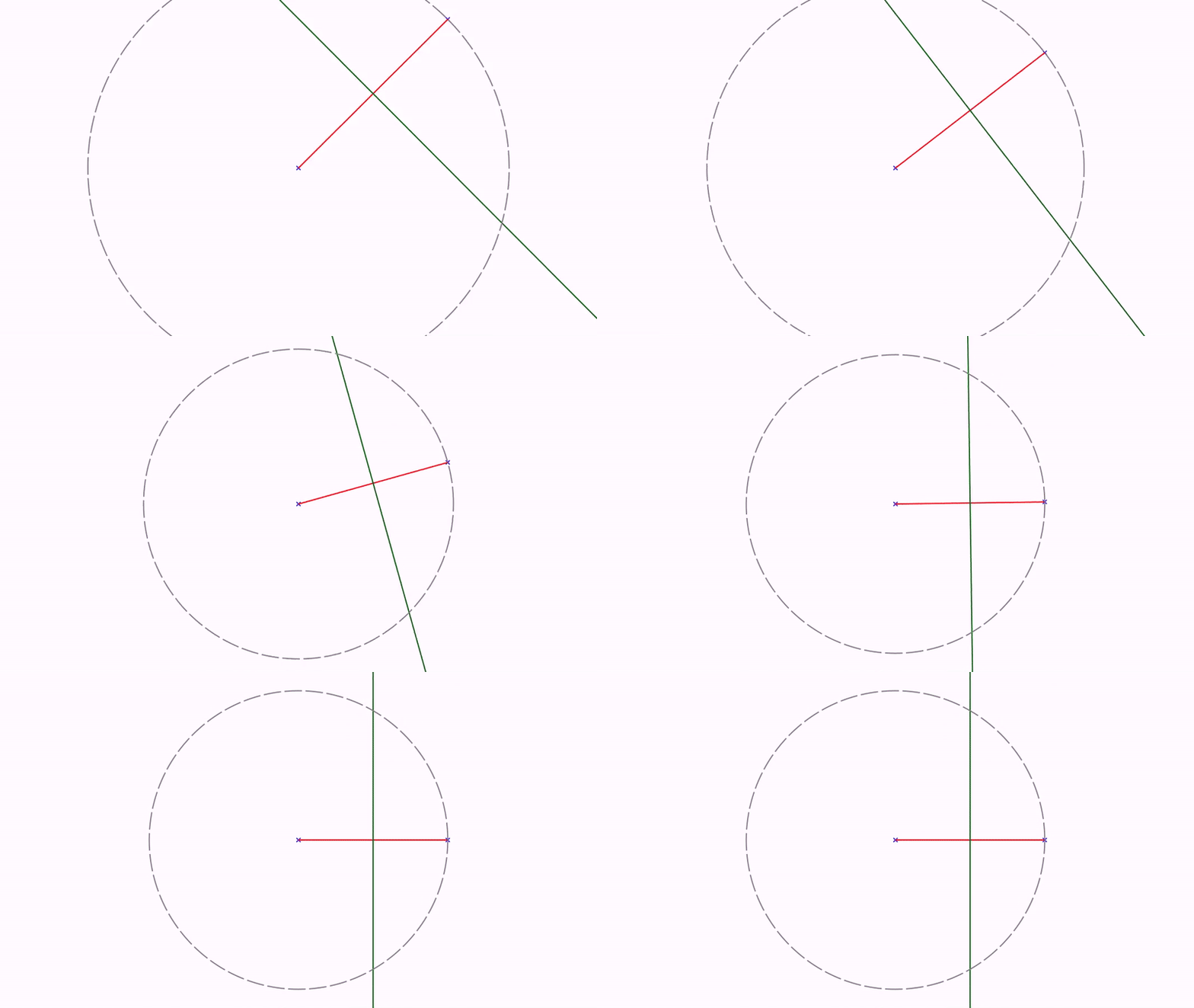
For example, the following code:
def A = ctPoint(
    at: [0, 0],
    style: [dotstyle: "cross", drawColor: 'blue']
)

def B = A + [1, 1] //copy of A shifted (1,1)

def segment = ctSegment(
    a: A,
    b: B,
    style: [thickness: 10, drawColor: 'red']
)

def perpBisector = ctPerpBisector(
    segment: segment,
    style: [drawColor: 'darkgreen', thickness: 10],
)
def circle = ctCircle(
    center: A,
    through: B,
    style: [dashstyle: "dashed", drawColor: 'gray']
)
scene.add(A, B, segment, perpBisector, circle)

animShift(
    runtime: 5,
    obj: B,
    vector: [0, -1]
)
 Or, if you prefer using Groovy syntax, the following code is equivalent:
def A = CTPoint.at(0, 0)
    .dotStyle(DotStyle.CROSS)
    .drawColor("blue")
def B = CTPoint.at(1, 1)
    .dotStyle(DotStyle.CROSS)
    .drawColor("blue")
def segment = CTSegment.make(A, B)
    .drawColor("red")
    .thickness(10)
def perpBisector = CTPerpBisector.make(segment)
    .drawColor("darkgreen")
    .thickness(10)
def circle = CTCircle.makeCenterPoint(A, B)
    .dashStyle(DashStyle.DASHED)
    .drawColor("gray")
scene.add(A, B, segment, perpBisector, circle)
play.shift(5, 0, -1, B)
In this example, we have created 2 CTPoint objects. These are almost identical to the classic Pointobject. The CTSegment object represents a segment between 2 CTPoint objects. Note that this object is not a Shape in the sense that you can transform it into another Shape for example, but it always remains as a segment. These objects are more rigid, but they allow for richer properties depending on the context.
The CTPerpBisector does as its name suggests, constructs the perpendicular bisector of the given segment.
Another object shown is the CTCircle. The static method makeCenterPoint(A,B) creates the circle with center A passing through point B.
Finally, we perform a shift animation to B. Note that all objects that depend on B are updated accordingly.
Each Constructible object has its own static constructor method with several parameters. For example, the CTPerpBisector allows a static constructor from a CTSegment but also with 2 CTPoint objects. Also, several builder methods that accept CTPoint are overloaded to accept Pointobjects (they simply wrap them into new CTPoint instances).
There are plenty of different Constructible, mostly trying to resemble Geogebra objects structure. In the snippet section of the graphic editor you can see all of them in the Objects/Constructible section, as they all have their DSL version implemented.
Naming a construction: name:
Every ct* builder takes a name:, the Geogebra-style label of the construction:
def A = ctPoint(at: [0, 0], name: "A")
def B = ctPoint(at: [2, 1], name: "B")
def r = ctLine(a: A, b: B, name: "r")
The name is not drawn on the screen: for that there is label:, described in
Labels. What it changes is the log, where the object is described by its name and its
inputs instead of by a bare list of coordinates:
r = CTLine[A, B]
Objects imported from a Geogebra file get the name they had there, which is what makes the log of
an import readable. A construction without a name is described by its type alone, CTLine[...].
Values in a construction: scalar
A construction is not only made of points and lines. The numbers it is built on, a radius, an
angle, a ratio, are scalar(...) objects, the very same ones a script animates. Written with
anything but a plain value:, a scalar is derived: computed from other objects and recomputed
whenever any of them changes, so whatever is built on it follows.
The form that carries the most is the written formula, evaluated by mXparser:
def t = scalar(0)
def r = scalar(expression: "1 + cos(t)", vars: [t: t])
def C = ctCircle(center: [0, 0], radius: r, addToScene: true)

animScalar(obj: t, from: 0, to: 2 * PI, runtime: 4)     // the circle breathes
Each name of vars becomes a variable of the formula. Another scalar is read live and declared as
an input of this one, so a change in it recomputes the value; a plain number is taken once as a
constant, since nothing can depend on it. The formula is mXparser's own syntax, so sin, cos,
ln, sqrt, pi, e and the rest of its vocabulary are available as they come.
The formula is checked when the scalar is built, not every time it is evaluated. A name the formula
uses and vars does not give, which is what a typo looks like, raises there and then instead of
quietly evaluating to NaN for the rest of the animation.
The other forms measure something of the construction:
def v = scalar(2.5)                       // a literal, same as scalar(value: 2.5)
def u = scalar(of: t)                     // follows another animatable value
def d = scalar(distance: [A, B])
def r = scalar(radius: circle)            // also an arc or a sector
def a = scalar(angle: [A, O, B])          // counterclockwise from A to B, in [0, 2*PI)
def s = scalar(area: poly)                // always positive, whatever the orientation
A derived scalar is read-only: its value comes from its own definition, so writing it, by hand or
with an animScalar, has no effect. Animate the values it is built on instead. A literal
scalar(value:) is the writable one, and the one to sweep.
Every parameter of a constructible builder that stands for a number takes a plain number or a scalar, and given a scalar the object goes on following it.
This is also the shape a locus needs. With the construction hanging from formulas, everything between the swept parameter and the traced point is recomputed on every sample.
Derived points
Besides a free point at given coordinates, ctPoint builds the points that other objects already
carry, or that follow from them. The type: parameter chooses which:
def O = ctPoint(type: "center", of: circle)     // also of an arc, a sector, an ellipse
                                                // or a regular polygon
def G = ctPoint(type: "centroid", of: poly)
def F = ctPoint(type: "focus", of: ellipse, index: 1)
def V = ctPoint(type: "vertex", of: poly, index: 2)
def P = ctPoint(type: "closest", on: segment, point: A)
Each one is a point of its own, with its own style and label, that follows whatever the object it
was read from does. Without type: you get the free point of the previous examples, so old scripts
keep working.
A word on two of them. The "centroid" is the center of mass of the region the polygon encloses,
not the average of its vertices: both agree for a triangle, but for any other polygon the average is
pulled towards wherever the vertices are more crowded. On a regular polygon the centroid is also the
center of the circumscribed circle, so there "center" and "centroid" give the same point. And the "closest" point respects the extent
of the object it projects on, so on a segment or a ray it stops at the ends and on an arc it stays
inside the arc. It is the passive counterpart of ctPointOnObject, which projects itself and can
therefore be dragged along the object.
Both accept any object able to hold a point: lines, rays, segments and vectors, circles, arcs, sectors and semicircles, function graphs, and polygons, regular polygons and polylines. On the last three the point lives on the outline and slides from one side to the next, so on a polyline, which is open, it stops at the two ends.
Vertices are numbered from 0. An ellipse has four of them: 0 and 1 are the ends of the major axis and 2 and 3 those of the minor one.
A point walking along a path: ctPointOnShape
The derived points above read something an object already carries. ctPointOnShape is different:
it lies anywhere on the path of another object, at the position a parameter says.
def sh = shape(type: "circle", transform: [scale: 2], addToScene: true)
def t = scalar(0)
def P = ctPointOnShape(shape: sh, t: t, style: [drawColor: "red"], addToScene: true)

animScalar(obj: t, from: 0, to: 1, runtime: 4)     // P goes once round the shape
shape: takes anything with a path, not only a Shape: a funcGraph, a parametricCurve, a
locus. The point follows both of its inputs, so animating t walks it along the path and moving
the path drags it with it.
t: accepts a plain number, and then the point sits there, but the form that matters is a
scalar(...): it is kept as it is, so whatever animates or sweeps that scalar moves the point. That
is what makes this the natural input of a locus.
The point recomputes itself from the path and the parameter, the way every constructible does, so a
locus can drive it, and nothing has to be written as an always updater, which the sweep would not
run.
The two ways of measuring the path
parametrized: chooses how t is spread along the path, with the same name and the same default as
animMoveAlongPath:
true, the default: by arc length.tis the fraction of the length covered and the point moves at constant speed. This is what "half way along the curve" means to a reader.false: by segment.tis spread evenly over the Bézier pieces the path is made of, however long each one is. Cheaper, and the way to land exactly on the vertices: on a rectangle with sides of 4 and 1,t = 0.25is the second corner withparametrized: false, and a point in the middle of the long side withparametrized: true.
Being constructible it is rigid, like the rest: shifting it does nothing, since the next pass
recomputes its position from the path. setFreeMathObject(true) detaches the drawn point when you
want to animate it on its own.
What the point knows about the curve under it
Besides where it is, the point answers what the curve is doing there:
| Method | What it gives |
|---|---|
getTangent() |
Unit vector along the curve, in the direction t grows |
getNormal() |
Unit normal, the tangent turned a quarter turn counterclockwise |
getCurvature() |
Signed curvature: positive where the curve turns left, zero on a straight piece |
getCurvatureRadius() |
Radius of the osculating circle, always positive, infinite where the curve is straight |
getCurvatureCenter() |
Centre of that circle, which is what an evolute traces |
getDerivative(), getSecondDerivative() |
The two derivatives everything above is built from |
def sh = shape(type: "circle", transform: [scale: 2], addToScene: true)
def t = scalar(0)
def P = ctPointOnShape(shape: sh, t: t)

println P.curvatureRadius        // 2, the radius of the circle
println P.curvatureCenter        // its centre
The curvature and everything derived from it belong to the curve, not to how it is measured, so the two parametrizations report the same number for the same place. The two derivatives are the exception: they are taken with respect to the Bézier parameter of the path, so their length says something about how the path is written and not about the curve it draws. What is geometric is their direction and the quantities above.
Three things to expect from a path made of Bézier pieces, all of which show up in an evolute:
- The curvature vanishes at an inflection and on a straight piece, and the centre of curvature
runs off to infinity there. The coordinates come back infinite, and a
locustracing them drops those samples and cuts the stroke, which is what the evolute of a straight piece should look like. - The second derivative jumps where two pieces meet, so the evolute genuinely breaks there.
maxJumpon the locus is what keeps that break from being drawn as a segment across the scene. - A point sitting exactly on such a joint reports a blend of the two sides, a couple of percent on a circle, since the difference is taken across the joint.
Constructible lines
The class CTAbstractLine has several subclasses such as CTLine, CTRay, CTSegment, CTAngleBisector, CTLineOrthogonal, CTPerpBisector, or CTVector. These are fairly self-explanatory, but one thing they have in common is that they all implement the interface HasDirection, which means that this object has an inherent direction (not oriented). So, we can use any of these objects as a parameter that admits a direction. For example, we can build a orthogonal line that passes through a CTPoint and is perpendicular to a CTLine, CTSegment, or CTVector. Other non-constructible objects, like Line, Ray or Arrow also implement this interface.
The CTAngleBisector admits two forms. Given three points, it builds the bisector of the angle they
determine, with the second point as the vertex. Given two lines, it builds one of the two bisectors
of the angle between them, chosen with the index: parameter: 0 halves the angle between the
directions of the lines as they are given, and 1 gives the other one, perpendicular to it. When
the two lines are parallel there is only one bisector, the line midway between them, and index: is
then ignored.
def bisABC = ctAngleBisector(a: A, b: vertex, c: C)
def bisLines = ctAngleBisector(line1: r, line2: s, index: 1)
Naming a line
Wherever a parameter stands for a straight line, any of these is accepted and they all mean the same thing:
axis: someCTLine        // or a CTSegment, a perpendicular bisector, any CTAbstractLine
axis: someLine          // a plain Line or Ray, read by the points defining it
axis: someSegmentShape  // a Shape with exactly 2 points
axis: [P1, P2]          // two points, or two raw pairs: [[0,0], [1,-1]]
Giving a constructible line keeps it as the input of what is built on it, so a line that is itself
derived from something else, a perpendicular bisector say, goes on being followed instead of being
flattened into two loose points. What is not accepted is a bare direction such as a Vec: it
tells which way the line runs but not where it is.
These are the parameters that take a line this way:
| DSL | Parameter |
|---|---|
ctAngleBisector |
line1:, line2: |
ctPerpBisector |
segment: |
ctMidPoint |
segment: |
ctMirrorPoint |
axis: |
ctTransformedLine |
line:, mirrorAxis: |
ctTransformedCircle |
mirrorAxis: |
ctParabola |
directrix: |
ctIntersectionPoint |
a:, b:, besides any other constructible |
ctPointOnObject, ctPoint(type: "closest") |
on:, besides any other object holding points |
affineTransform, animAffine with type: "reflectionByAxis" |
axis: |
A dir: parameter asks for a direction and not for a line, so it takes all of the above and a
bare direction, that is, a Vec or a raw [x, y] pair. ctLine, ctRay, ctLineOrthogonal,
ctParabola, line and ray have one:
def r = ctLine(a: A, dir: [1, 1])            // a bare direction
def r = ctLine(a: A, dir: someSegment)       // the direction of something that runs along one
def r = ctLine(a: A, dir: [P1, P2])          // or of the line two points define
Conics
Besides circles and their arcs, the three remaining conics are built from their foci:
def e = ctEllipse(focus1: F1, focus2: F2, a: P)      // through P
def h = ctHyperbola(focus1: F1, focus2: F2, a: P)    // both branches
def p = ctParabola(focus: F, directrix: d)           // see above for what d may be
def p = ctParabola(focus: F, a: P1, dir: v)          // directrix through P1 along v
The directrix: is a line parameter, so it takes every form
a line may be written in, and a: plus dir: is the form that takes a bare
direction, which no line parameter accepts.
An ellipse is a closed curve and there is nothing to decide about it, but a parabola and a
hyperbola run to infinity, so how far to draw them is not a property of the curve: it is
decided by the camera. Both generate only the part that fits in the current view and recompute
it whenever the camera moves, exactly as an infinite Line does. Consequently they are also
left out of the box the camera fits itself to, the same way lines and rays are, since a curve
that stretches to fill the view and a camera that adjusts to its objects would chase each other.
That is the right behaviour while the scene is still, but not while an animation is transforming
or drawing one of them and the camera is moving at the same time: the points would be shifting
underneath. The trange: parameter pins the interval of the parameter instead, and the curve
stops following the camera:
def p = ctParabola(focus: F, directrix: d, trange: [-4, 4])
def h = ctHyperbola(focus1: F1, focus2: F2, a: P, trange: [-2, 2])
For the parabola the parameter is the signed distance to its axis, so 0 is the vertex. For the
hyperbola each branch is drawn as (a·cosh t, b·sinh t) in its own frame, so 0 is its vertex
and both branches get the same interval.
A parabola is drawn with a single cubic Bézier and it is exact, not an approximation, however long the arc: written in its own frame the curve is a polynomial of degree two, and every polynomial curve of degree at most three is a Bézier. A branch of a hyperbola is not a polynomial, so it is approximated by a fixed number of cubic pieces; the interval of the parameter only grows as the logarithm of the zoom, so the error stays well under a pixel however far the camera pulls back.
Both hold points, like the rest of constructible objects, so ctPointOnObject works on them. The
point is projected onto the whole curve and not only onto the arc currently visible, which is why
it may end up off screen.
All four conics also know how to write themselves as an implicit equation, and two things follow
from that alone. One is meeting a line, which is a plain quadratic, so ctIntersectionPoint
works against any of them (index 0 is the intersection nearer to the first point of the line,
1 the other one; see CTIntersectionPoint for what the index counts when
the straight object is a ray or a segment). The other is the tangent from a point, which is the polar line: when the
point lies on the curve the polar is the tangent there, and when it lies outside it joins the two
points of contact, so one computation covers both cases.
def p1 = ctIntersectionPoint(a: someLine, b: par, index: 0)
def t0 = ctTangent(point: P, conic: par)          // touches at one point
def t1 = ctTangent(point: P, conic: par, index: 1)  // and at the other
A point inside the conic has no real tangent, and the line then reports it the way the rest of the library does: its second point comes back as NaN. Intersecting two conics is not supported; that is a quartic and not a quadratic.
CTLaTeX
Mostly like his brother-in-code, LatexMathObject, this object represents a LaTeX string to be drawn on screen. This object is permanently stacked at a given CTPoint. We'll see an example of this class in the next section.
CTIntersectionPoint
The CTIntersectionPoint object extends the CTPoint object and represents the intersection point between two constructible objects. In the current version, several static builders can be used:
CTIntersectionPoint p1=CTIntersectionPoint.make(ct1,ct2,num);
Where ct1 and ct2 can be any straight object (CTLine, CTSegment, CTRay), any circle or
circle part (CTCircle, CTCircleArc, CTCircleSector, CTSemiCircle, the circumcircle ones and
CTTransformedCircle) or any conic (CTEllipse, CTParabola, CTHyperbola). Meeting a circle or
a conic may give 2 points, and the num variable (0 or 1) determines the solution number.
In the DSL, a: and b: take a constructible object as above, and also a straight line written in
any of the forms a line parameter accepts, so a: someLine or a: [P1, P2] work
too.
What the index counts
The index numbers the intersections that really exist, and not the roots of the equation. Half of the objects here are only part of the curve they lie on, and a root that falls on the rest of it is not an intersection of the objects that were given:
- a ray drops what falls behind its origin, and a segment what falls past either end;
- an arc, a sector or a semicircle are only met where they are drawn, never on the rest of their circle.
So index 0 is always the first point one can actually see. A ray leaving the vertex of an angle
and crossing the arc that marks it gives that crossing at index 0, even though the line the ray
runs along cuts the circle behind the vertex as well.
When there is no intersection at all, or fewer than the index asks for, the point comes back with NaN coordinates, which is how the rest of the library reports a construction that has nothing to show. Two tangent objects count as meeting, and give the same contact point at both indices.
Intersecting two conics other than circles is not supported: that is a quartic and not a quadratic.
For example, the following code:
def A=ctPoint(
    at: [.3,0],
    style: [drawColor: 'blue']
)
def B=ctPoint(
    at: [-.5,-.1],
    style: [drawColor: 'red']
)

def lineAB = ctLine(
    a: A,
    b: B
)
def circle = ctCircle(
    center: [0,0],
    radius: 1
)

def inter1=ctIntersectionPoint(
    a: circle,
    b: lineAB,
    index: 0,
    style: [drawColor: 'green']
)
def inter2=ctIntersectionPoint(
    a: circle,
    b: lineAB,
    index: 1,
    style: [drawColor: 'orange']
)

scene.add(A, B, lineAB, circle, inter1, inter2)


ctLatex(text: r"$A$",anchor: A, anchortype: "diag4",gap: .3, scale: .5,addToScene: true)
ctLatex(text: r"$B$",anchor: B, anchortype: "diag4",gap: .3, scale: .5,addToScene: true)
ctLatex(text: r"$0$",anchor: inter1, anchortype: "upper",gap: 1, scale: .5,addToScene: true)
ctLatex(text: r"$1$",anchor: inter2, anchortype: "upper",gap: 1, scale: .5,addToScene: true)

animShift(
    runtime: 2,
    obj: B,
    vector: [0,-.5]
)
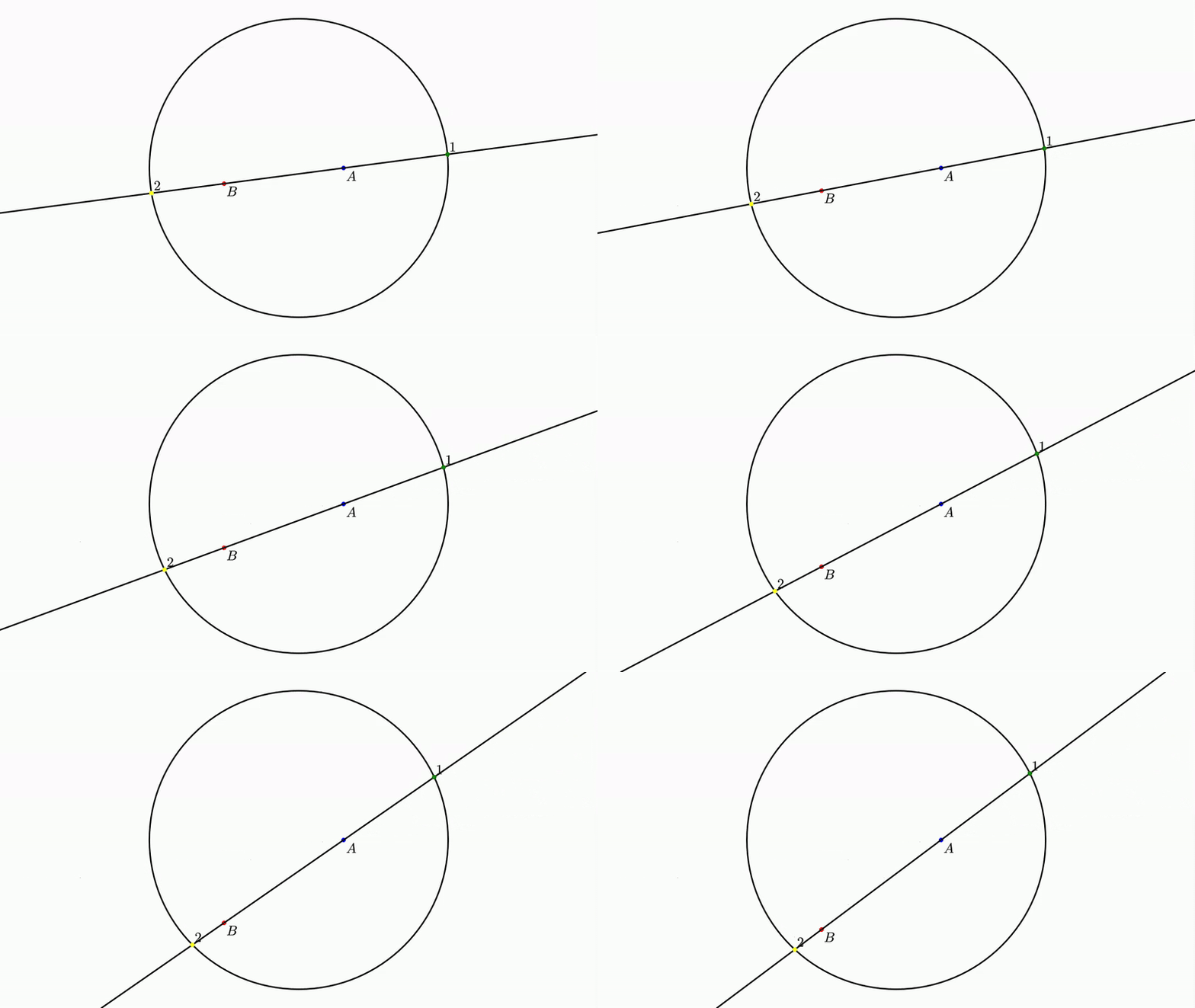
It generates the following image with the 2 solutions numbered. Which solution number should we choose? If we parametrize the line AB where A is at t=0 and B is at t=1, and the intersections are located at parameter t1 and t2, then solution number 0 is at min(t1,t2) and number 1 is at max(t1,t2):
If there is no intersection, the point returned will have coordinates Double.NaN. You can check if any of the coordinates a point is NaN with the method isNaN().
def P=....
    if (P.isNaN()) {
        //Sorry mate, at least one coordinate is NaN...
    }
Polygons and triangles
ctPolygon builds a polygon in two ways: from the list of its vertices, or as a regular polygon
given one side and the number of sides. In the regular form only A and B are inputs, and the
remaining vertices are computed from them.
def poly = ctPolygon(points: [A, B, C, D])
def hex  = ctPolygon(A: A, B: B, sides: 6)
ctTriangle chooses its construction from the parameters it is given:
| Parameters | What is built |
|---|---|
A:, B:, C: (or points: [A, B, C]) |
The triangle with those 3 vertices, all of them inputs |
A:, B:, angleA:, angleB: |
The triangle resting on the side AB with those interior angles |
sideAB:, sideBC:, sideCA: |
The triangle with those side lengths, placed at the origin |
sideAB:, angleA:, angleB: |
The same, with the other two sides given by the two angles |
sideAB:, sideBC:, angleB: |
Two sides and the angle they form |
sideAB:, sideBC:, angleA: |
Two sides and the angle BC does not rest on, plus index: |
any length form + A: and/or angle: |
The same triangle, resting on that point and direction |
def t  = ctTriangle(A: [0, 0], B: [1, 0], C: [1, 1])
def eq = ctTriangle(A: [0, 0], B: [1, 0], angleA: PI/3, angleB: PI/3)
def eq2 = ctTriangle(sideAB: 1, angleA: PI/3, angleB: PI/3)
The two forms that give a side by its two ends rest on those points, and follow them. The forms that give the sides as lengths do not depend on any point, so they are placed on their own, which is described below.
Giving only one of the two angles, or an angle together with C, is an error: the first leaves the
triangle undetermined and the second overdetermines it.
Every form that computes a vertex follows the same convention: the given side runs from left to
right and the computed vertex lies above it. Angles are in radians, and like every numeric
parameter of a construction they also accept a scalar(...), so they can be animated:
def angle = scalar(PI/6)
def t = ctTriangle(A: [0, 0], B: [2, 0], angleA: angle, angleB: PI/4, addToScene: true)
animScalar(obj: angle, to: PI/2, runtime: 3)
Reading the vertices and the perimeter
Every constructible polygon, polyline and triangle gives its vertices and the points of its perimeter the same way:
def v = t.getVertex(0)        // the vertex object itself, so what is built on it follows
def v = t[0]                  // the same, and t[-1] is the last one
def p = t.getParametrized(.5) // point halfway round the perimeter, measured along its length
def p = t(.5)                 // the same
def q = t.get(.5)             // point at half the path, every side taking the same share
getVertex returns the vertex itself and not a copy, so a ctPoint, a label or another
construction built on it follows the polygon. The two positions differ only when the sides have
different lengths: get splits the parameter evenly between the sides, getParametrized splits
it by length.
The notable points, lines and circles
A ctTriangle builds its own notable elements, so they do not have to be composed by hand out of
bisectors and intersections:
| Method | What it gives |
|---|---|
getSide(n) |
The side n as a segment. Side 0 is AB, side 1 is BC, side 2 is CA |
getMedian(n) |
Segment from the vertex n to the midpoint of the opposite side |
getAltitude(n) |
Line through the vertex n perpendicular to the opposite side |
getPerpBisector(n) |
Perpendicular bisector of the side n |
getAngleBisector(n) |
Interior angle bisector at the vertex n |
getCentroid() |
Where the three medians meet |
getIncenter() |
Where the three angle bisectors meet |
getCircumcenter() |
Where the three perpendicular bisectors meet |
getOrthocenter() |
Where the three altitudes meet |
getIncircle() |
Circle tangent to the three sides |
getCircumcircle() |
Circle through the three vertices |
def tri = ctTriangle(A: [0, 0], B: [4, 0], C: [1, 3])
scene << tri << tri.getMedian(0) << tri.getCentroid() << tri.getCircumcircle()
Each of them is built the first time it is asked for and kept, so asking twice gives the same
object back and reading one from an updater costs nothing. Vertex and side indices count from 0
and from the end when negative, the same as getVertex.
The altitudes are lines and not segments because in an obtuse triangle the foot of an altitude falls outside the side it is perpendicular to. For the same reason the orthocenter can lie outside the triangle, and in a right triangle it sits on the vertex of the right angle.
The three notable points and the two circles are also reachable from the DSL:
def I = ctPoint(type: "incenter", of: tri)        // also "circumcenter" and "orthocenter"
def c = ctCircle(inscribedIn: tri)
def C = ctCircle(circumscribedTo: tri)
The rest are read as methods. The lines they stand for can also be built with ctPerpBisector,
ctAngleBisector and the other line constructibles, taking the vertices with tri[0], tri[1]
and tri[2].
The angles and the sides as scalars
getAngle(n) and getSideLength(n), and the named angleA, angleB, angleC, sideAB,
sideBC and sideCA, answer with a scalar(...):
def tri = ctTriangle(sideAB: 1, sideBC: 1, angleB: 80*DEGREES)
animScalar(obj: tri.angleB, to: 30*DEGREES, runtime: 3)   //the angle drives the triangle
When the form that built the triangle takes that number, what you get back is the very scalar the
construction is driven by, so writing or animating it moves the triangle, exactly as if you had
declared it yourself with scalar(...). When it does not, the scalar is derived from the vertices:
it follows the triangle, and writing it logs a warning and does nothing, which isDerived()
reports in advance.
def t = ctTriangle(A: [0, 0], B: [4, 0], C: [0, 3])
t.angleA.value          // PI/2, derived from the vertices
t.angleA.isDerived()    // true: this form is not defined by its angles
t.sideAB.value          // 4
So they are always readable, which is what a label showing a measurement needs, and writable exactly when it makes sense. Declaring the scalar yourself is still the better style when two objects share it, because then it belongs to the construction and not to one triangle.
The ambiguous case
sideAB, sideBC and the angle at B, the one the two sides form, always determine one
triangle. The angle at A, which the side BC does not rest on, does not: depending on the
numbers there are two triangles, one, or none at all, which is why two sides and a non-included
angle are not a criterion of congruence. index: picks which one, 0 for the triangle with the
shorter side CA and 1 for the longer one, the same way ctIntersectionPoint numbers its
solutions.
def sas  = ctTriangle(sideAB: 3, angleB: PI/2, sideBC: 4)          //one triangle, the 3-4-5
def one  = ctTriangle(sideAB: 2, sideBC: 1.2, angleA: PI/6, index: 0)
def two  = ctTriangle(sideAB: 2, sideBC: 1.2, angleA: PI/6, index: 1)
Animating the length of BC is the classic picture of the case: while it is shorter than the distance from B to the other side of the angle neither triangle exists and both are drawn empty, they appear together when it reaches it, separate as it grows, and the first one disappears when BC becomes as long as AB.
A rigid triangle that can still be moved
A triangle given by its three side lengths has a shape but no place to be, so it is the one constructible object that owns where it sits: A starts at the origin, B to its right, and the third vertex is computed from the lengths.
def t = ctTriangle(sideAB: 3, sideBC: 4, sideCA: 5, addToScene: true)
t.shift(1, 2).rotate(PI/6)
animShift(obj: t, vector: [2, 0], runtime: 2)
Because of that it takes shifts, rotations and reflections like an ordinary MathObject, which
no other constructible does: the transform is absorbed into its placement instead of being
ignored. A scale relocates it but never resizes it, since the lengths are its inputs and nothing
writes them. To animate the size, animate the lengths themselves:
def side = scalar(4)
def t = ctTriangle(sideAB: 3, sideBC: side, sideCA: 5, addToScene: true)
animScalar(obj: side, to: 6, runtime: 3)
Give it a placement to rest on, A: or angle: or both, and it goes back to behaving like every
other constructible: it follows those objects through the dependency graph and ignores transforms
of its own.
def P = ctPoint(at: [1, 1])
def t = ctTriangle(A: P, angle: PI/4, sideAB: 3, sideBC: 4, sideCA: 5)
Degenerate parameters
While the parameters do not define a triangle, for instance when the two angles add up to a straight angle or when one side is longer than the other two together, the object is drawn empty and a warning is logged. It comes back on its own as soon as the parameters define it again.
Labels
Every constructible object, except ctLatex, takes the same inline label: parameter as the rest
of the DSL, and places it on the object it draws: on the dot for a point, along the path for a
line, a segment, a circle or a conic.
def A = ctPoint(at: [0, 0], label: r"$A$")
def B = ctPoint(at: [2, 0], label: r"$B$")
def s = ctSegment(a: A, b: B, label: [text: r"$c$", t: 0.5])
def c = ctCircle(center: A, through: B, label: [text: r"$\Gamma$", t: 0.25])
def p = ctPolygon(points: [A, B, P], label: [r"$a$", r"$b$", r"$c$"])
The label is registered as an internal object of the constructible, so it is updated, drawn and
animated with it and must never be added to the scene on its own. That is exactly what a
construction wants: drag a defining point and every label of every object depending on it is
placed again. Labels can be restyled by name with parts: [label0: [color: "red"]] and read back
with getLabel(), getLabel("key") or getLabel(0).
The full catalog of label options is in the Adding labels chapter.
Converting to non-constructible MathObjects
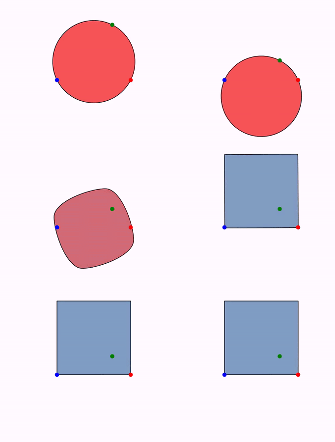
Suppose you have built a CTCircle that passes through 3 points, but now you want to transform it into a square. You cannot do that with a Constructible object (in fact, it will give you an error), but you can extract the contained MathObject which is actually drawn and perform any transformation to it.
//With the layer(1) we ensure the dots are over the rest of the objects
def A = ctPoint(
      at: [0, 0],
      style: [drawColor: 'blue', thickness: 60, layer: 1]
)
def B = ctPoint(
      at: [1, 0],
      style: [drawColor: 'red', thickness: 60, layer: 1]
)
def C = ctPoint(
      at: [.75, .75],
      style: [drawColor: 'green', thickness: 60, layer: 1]
)
def circle = ctCircle(
      a: A,
      b: B,
      c: C,
      style: "solidred"
)

scene.add(A, B, C, circle)

//Let's move the C point for fun!
animShift(
    runtime: 2,
    obj: C,
    vector: [0,-.5]
)

//The next command is necessary! Doing so it will remove an unused object from the scene
//but more importantly, it will unregister the CTCircle from the update queue
//and stop updating the contained MathObject, leaving it "free".
scene.remove(circle)

def shape = circle.getMathObject()
morph(
    type: "auto",
    from: shape,
    to: Shape.square().style("solidblue")
)

scene.waitSeconds(3)
Geogebra import
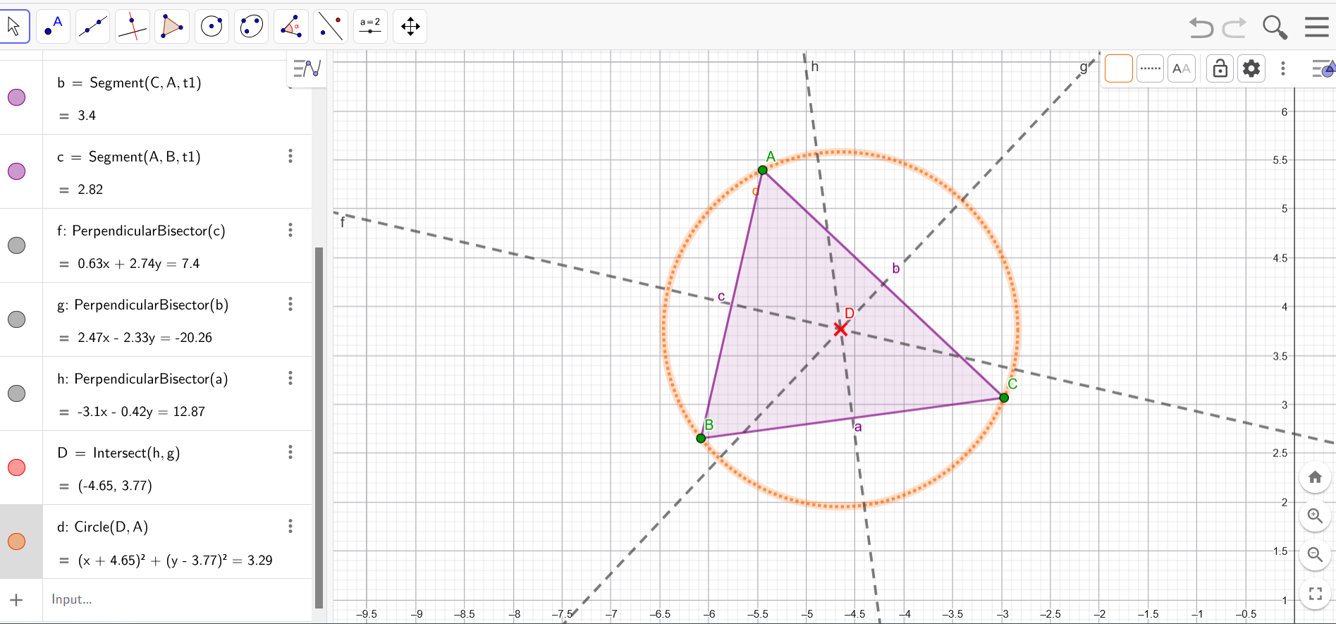
One of the advantages of Constructible objects is that they behave similarly to the objects of the Geogebra program. In the rare case you don't know it, Geogebra is an excellent open source software that allows you to do geometric constructions (and many other things). JMathAnim can import Geogebra files in a limited way (keep in mind that Geogebra has literally hundreds of commands!). For now, the following elements can be successfully imported: points, midpoints, intersections (of lines, rays, segments, circles), lines, orthogonal, parallel, perpendicular bisectors, polygons, regular polygons, vectors, mirrored, translated, and rotated points. JMathAnim will log a warning when it finds an unknown command that cannot be imported. The process is quite simple. For example, suppose we have a document like this created in Geogebra, where we have calculated the circumcenter of a triangle, drawing the 3 perpendicular bisectors:
Now, we save this in our disk under the name test.ggb, in a directory named resources/geogebra of our project. This will be the default location for Geogebra files (remember, you can change this behavior with the # and ! flags).
//With this command we parse the file resources/geogebra/test.ggb
def gl = GeogebraLoader.parse("test.ggb")
Now, JMathAnim will try to convert all Geogebra elements, logging a warning if there is an unknown command (and possibly throwing an exception if there are objects that depend on this unknown object). If all goes well, the gl object will have a Dictionary with the created objects.
The command
scene.add(gl)
This is equivalent to adding all the imported objects to the scene.
If you want to adjust the camera to the view of the original Geogebra document, you can do this with the command:
camera.setViewFrom(gl)
Note that the proportions of JMathAnim's and Geogebra's mathviews may not be the same, so the view is approximate.
The imported document will look like this:
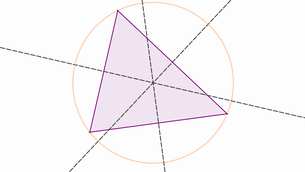
Not bad, right? Note that axis and object labels are not imported. And that's it! Well, not really. If you want to animate elements or simply access to them, you can use the original names that these objects had in Geogebra. For example, to access point A, you can use the command
gl.get("A");
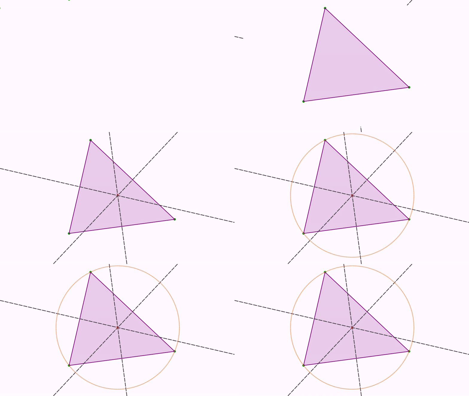
 //With this command we parse the file resources/geogebra/test.ggb
def gl = GeogebraLoader.parse("test.ggb");
camera.setViewFrom(gl)
play.run(
    Commands.moveIn(1, ScreenAnchor.LEFT, gl.get("A")),
    Commands.moveIn(1, ScreenAnchor.UPPER, gl.get("B")),
    Commands.moveIn(1, ScreenAnchor.RIGHT, gl.get("C"))
);
play.showCreation(gl.get("t1"))
play.showCreation(gl.get("f"), gl.get("g"), gl.get("h"))
play.moveIn(ScreenAnchor.UPPER, gl.get("D"))
play.showCreation(gl.get("d"))
scene.waitSeconds(1)
play.contourHighlight(gl.get("D"))
Limitations
Currently JMathAnim can import most common geometric constructions, but there are other elements that cannot be imported yet. For example, any element that is built from an algebraic expression given in a string cannot be imported. This applies to functions or points whose coordinates are not numbers but formulas.