Calculus objects
This chapter gathers the objects you reach for when your animation is about functions and fields rather than plain shapes:
funcGraph: the graph $y=f(x)$ of a single-variable function.pointOnGraph: a point that rides along a function graph.contourPlot: the level curves of a scalar field $f(x,y)$.densityPlot: a scalar field $f(x,y)$ painted as a colored heat-map.vectorField: a planar vector field $F(x,y)$ drawn as a grid of arrows.
Function graphs are simple enough to write either way, but the field objects (contour, density, vector) are powerful, and that power comes at a price: they have a lot of arguments (domain, grid resolution, color scale, arrow style, coordinate system...). Writing them the "raw Groovy" way means juggling constructors with six or seven positional arguments, and remembering the order.
So in this chapter we lead with the DSL format, where every option has a name and you only write the ones you care about. It reads almost like plain English and the editor autocompletes it for you. Where useful, we include a small "In plain Groovy" note showing the equivalent object-oriented code, but for these objects the DSL really is the comfortable way to travel.
Let the editor do it: every command below lives in the snippets palette (
Alt+S, or the sidebar). Insert the block, then pressCtrl+Spaceinside it to see and add the available parameters, each with a short description. You never have to memorize the tables below.
The field objects (contourPlot, densityPlot, vectorField) all share the same spirit:
- If you omit the domain (
rect), they use the current camera view. - They can be recolored through a
colorScale. - If the function takes an additional parameter
t, they become animatable (see Animating a field).
Table of Contents
- funcGraph
- pointOnGraph
- contourPlot
- densityPlot
- vectorField
- Animating a field
- A value of your own: scalar
- Showing the value: slider
- Building lists of levels: linspace and arange
funcGraph
The most everyday calculus object: the graph of a one-variable function $y=f(x)$. You pass the function as a closure ({ x -> ... }, see the Groovy survival kit if closures are new to you):
def fg = funcGraph(func: { x -> Math.sin(x) })
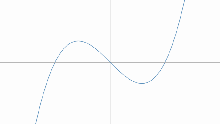
With no range given, the graph is dynamic: it spans whatever the camera currently shows and redraws itself if you pan or zoom. Give an explicit xRange to pin it to a fixed interval, and style it as any other shape:
axes()
def fg = funcGraph(
    func:   { x -> x*x*x - x },
    xRange: [-1.5, 1.5],
    style:  [drawColor: "steelblue", thickness: 8]
)
scene.add(fg)
Parameters at a glance
| Key | What it does |
|---|---|
func |
The function { x -> ... } (required) |
xRange (or range) |
Domain [from, to]. Omitted → dynamic, follows the camera |
numPoints |
Number of sample points (only meaningful with an explicit range) |
dynamic |
Force a dynamic range even when xRange is given |
style, label |
Style map and inline label(s), as in any shape |
In plain Groovy:
funcGraph(func: { x -> Math.sin(x) }, xRange: [-3, 3])is equivalent toFunctionGraph.make({ x -> Math.sin(x) }, -3, 3). The dynamic version is justFunctionGraph.make({ x -> Math.sin(x) }).
A FunctionGraph is a full Shape under the hood, so it supports showCreation, transform, MoveAlongPath and everything else. Because it appears so often in examples across this manual (it's the star of the lambda-visualization gallery in the animation effects chapter), it is worth getting comfortable with.
Parametric and polar curves. For curves that aren't graphs of a function (circles, spirals, roses), use the sibling parametricCurve(...) command, which takes x/y closures (or r/theta for polar) and a trange:
def rose = parametricCurve(r: { t -> Math.cos(3*t) }, theta: { t -> t }, trange: [0, PI])
pointOnGraph
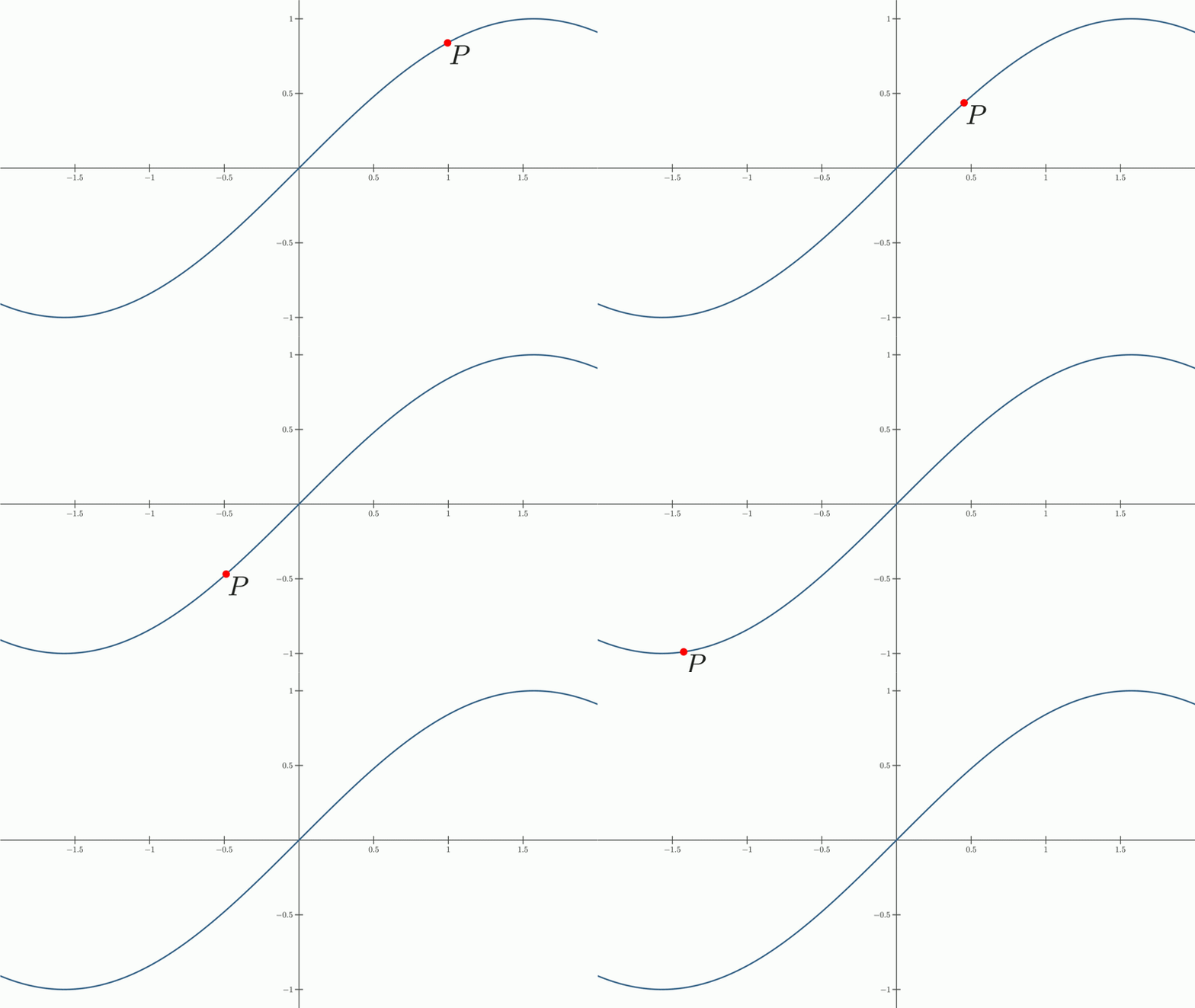
A pointOnGraph is a point that lives on a function graph: its $y$ coordinate is always $f(x)$, and it recomputes itself every frame. The magic is that shifting it horizontally makes it slide along the curve (perfect for "let this point travel along the graph" animations, or for anchoring a label to a moving spot on a function).
axes(
        xRange: [-5, 5],
        yRange: [-5, 5],
        xStep: .5,
        yStep: .5
)
def fg = funcGraph(
        func: { x -> Math.sin(x) },
        addToScene: true,
        style: [drawColor: 'steelblue4', thickness: 10])

def p = pointOnGraph(
        x:     1,
        graph: fg,
        style: [color: "red", dotStyle: "circle", thickness: 50],
        label: r"$P$",
        addToScene: true
)
// Slide the point from x=1 to x=1-4=-3 along the sine curve
play.shift(4, -4, 0, p)
Parameters at a glance
| Key | What it does |
|---|---|
x |
Initial x coordinate of the point along the graph (required) |
graph |
The funcGraph the point rides on (required; aliases funcGraph, on) |
style |
Style map, e.g. [color: "red", dotStyle: "circle", thickness: 4] |
label |
Inline label(s), exactly as in point(...): "$P$" or a map/list of specs |
addToScene |
Add to the scene immediately (default false) |
The difference from a normal Point is that a pointOnGraph stays on the curve no matter what. Animate its x, animate the underlying function, zoom the camera, the point tracks f(x) throughout, and any label attached to it comes along for the ride. It also exposes the neighbouring slope points (getSlopePointRight() / getSlopePointLeft()), which are handy control points if you want to draw a tangent line or segment at the moving point.
In plain Groovy:
pointOnGraph(x: 1, graph: fg)isPointOnFunctionGraph.make(1, fg).
contourPlot
Draws the level curves of a scalar field f(x,y) (the lines where f(x,y)=c for each level c), using the Marching Squares algorithm. Each contour line is an independent shape, so the whole thing can be styled, colored and animated as one.
The simplest possible call needs only the function and the levels:
def cp = contourPlot(
    function: { x, y -> x*x + y*y },     // f(x,y) = x² + y²
    levels:   [0.2, 0.7, 1.0]            // draw the curves f = 0.2, 0.7 and 1.0
)
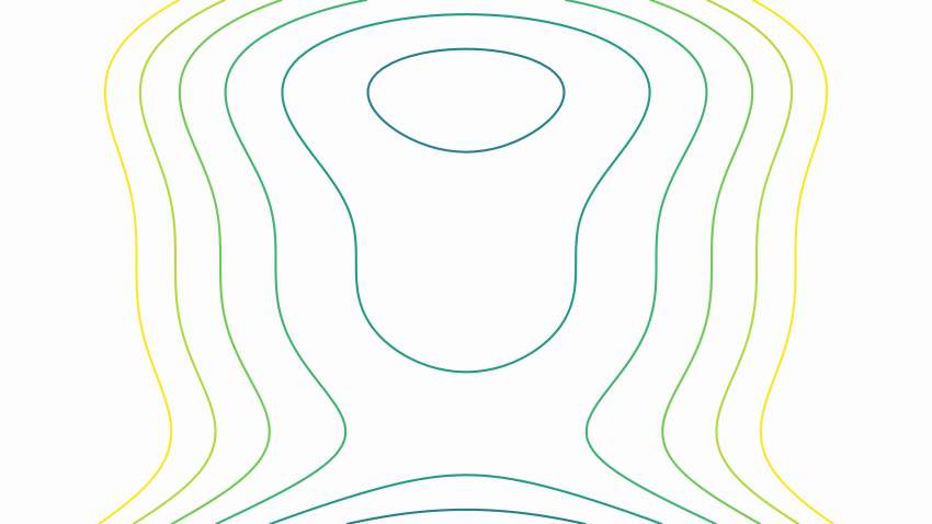
Since the domain was omitted, the contours are computed over whatever the camera is currently showing. A richer example, with an explicit domain, a finer grid and a color scale:
scene.add(Axes.make())
def cp = contourPlot(
    function: { x, y -> (1 + x*x) / (1 + y*y*y*y) },
    levels:   [min: 0.5, max: 3.0, step: 0.5],   // levels 0.5, 1.0, ... 3.0
    rect:     [-3, -3, 3, 3],                    // xmin, ymin, xmax, ymax
    cols: 150, rows: 150,                        // grid resolution
    colorScale: [["blue", 0], ["white", 1.5], ["red", 3]]
)
Parameters at a glance
| Key | What it does |
|---|---|
function |
The scalar field { x, y -> ... } (required) |
levels |
The list of contour values. A plain list [0.5, 1, 1.5], or a [min:.., max:.., step:..] map, or a linspace/arange call (see below) |
rect |
Domain [xmin, ymin, xmax, ymax]. Also accepts a preset name ("unit", "centered", "screen", "trig", "trigCentered") or a single number n for a centered $[-n,n]^2$ square. Omitted → camera view |
cols, rows |
Grid resolution (default 100). Higher = smoother curves, slower |
colorScale |
Colors the contours by their level value (list of [color, value] stops, or a colorScale(...)) |
style |
A style map applied to every contour shape |
In plain Groovy: the DSL call above is equivalent to building the object and its color scale by hand:
def cp = ContourPlot.make(
    { x, y -> (1 + x*x)/(1 + y*y*y*y) },
    -3, 3, -3, 3, 150, 150,
    0.5, 1.0, 1.5, 2.0, 2.5, 3.0)
def sc = ColorScale.make().add(0, "blue").add(1.5, "white").add(3, "red")
cp.applyColorScale(sc)
scene.add(cp)
Same result, more parentheses to count.
densityPlot
Paints a scalar field f(x,y) as a colored raster (a heat-map): every pixel is evaluated and its value mapped through a color scale. Unlike contourPlot, this is a bitmap, so it doesn't produce individual curves.
densityPlot adds itself to the scene automatically, so you don't even need scene.add:
densityPlot(function: { x, y -> Math.sin(x) * Math.cos(y) })
If no color scale is given, it builds a default viridis scale spanning the actual range of values it finds. A more explicit call:
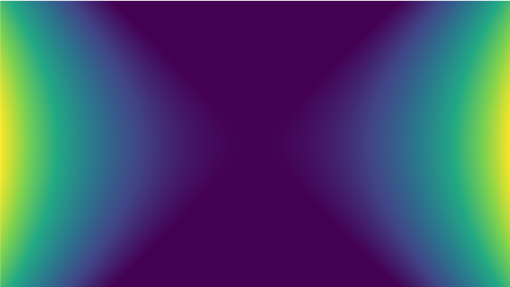
def dp = densityPlot(
    function:   { x, y -> x*x - y*y },
    rect:       [-2, -2, 2, 2],
    colorScale: ["viridis", 0, 4]      // viridis scale mapped to values 0..4
)
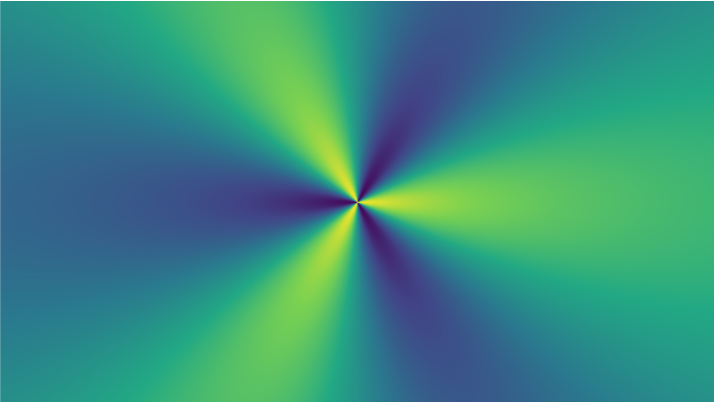
Polar mode. Set coordinates: "polar" and your function receives (r, theta) instead of (x, y):
densityPlot(
    function:    { r, theta -> Math.cos(3*theta) / (1 + r) },
    coordinates: "polar"
)
Parameters at a glance
| Key | What it does |
|---|---|
function |
The scalar field { x, y -> ... } (or { x, y, t -> ... } to animate) (required) |
rect |
Domain, same options as in contourPlot. Omitted → camera view |
coordinates |
"cartesian" (default) or "polar" (function gets r, theta) |
colorScale |
The color scale. A ["viridis", min, max] shorthand, or a colorScale(...) |
style |
Mainly the fill opacity, e.g. [alpha: 0.6] |
In plain Groovy: the first example is equivalent to
def dp = DensityPlot.make(Rect.make(-2, -2, 2, 2)) { x, y -> x*x - y*y }
dp.setColorScale(ColorScale.viridis(0, 4))
scene.add(dp)
and there are
dp.polar()/dp.cartesian()methods to toggle the coordinate mode after creation.
vectorField
Draws a planar vector field F(x,y) as a grid of arrows. Like contourPlot, each arrow is an independent shape, so styling and animations apply to the whole field at once. It also adds itself to the scene automatically.
The field function returns the vector at each point, either as a Vec or as a plain [vx, vy] list:
vectorField(function: { x, y -> Vec.to(Math.sin(PI*x), Math.cos(PI*y)) })

// The same, returning a plain list
vectorField(function: { x, y -> [Math.sin(PI*x), Math.cos(PI*y)] })
Both give the same image:
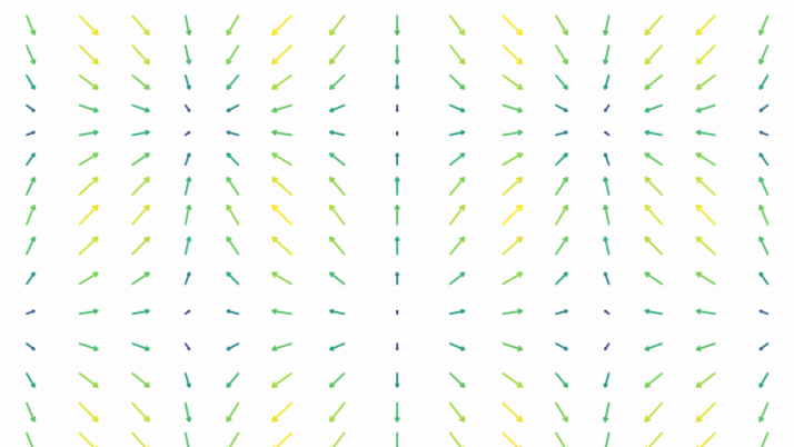
the vectorField method uses a special class of lightweight arrows. If you want to use "classic" arrows as we saw in previous chapters, just specify the value arrows: "classic".
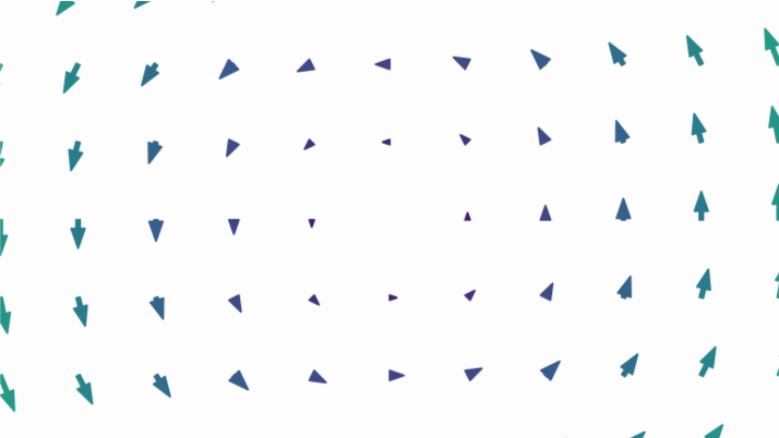
A fuller example with a finer grid, filled arrowheads and per-magnitude coloring:
def vf = vectorField(
    function: { x, y -> Vec.to(-y, x) },
    rect:     [-3, -3, 3, 3],
    cols: 20, rows: 20,
    arrows:   "classic",         // filled arrowheads (prettier, a bit slower)
    colorByMagnitude: true       // color each arrow by its length, viridis scale
)
Parameters at a glance
| Key | What it does |
|---|---|
function |
The field { x, y -> Vec.to(...) } (or a [vx, vy] list; add a third t to animate) (required) |
rect |
Domain, same options as in contourPlot. Omitted → camera view |
cols, rows |
Grid resolution (default 15) |
arrows |
"simple" (stroke-only, default) or "classic" (real filled heads) |
normalize |
true draws every arrow the same length (direction only) |
scaleFactor |
Fraction of a grid cell the longest arrow occupies (default 0.9) |
lengthScale |
Fixed world-length per unit magnitude (turns off auto-scaling) |
colorByMagnitude |
true auto-colors arrows by magnitude with a viridis scale |
colorScale |
A custom color scale for the magnitude coloring |
style |
A style map applied to every arrow |
By default arrow lengths are auto-scaled so the longest one fits neatly inside a grid cell without stepping on its neighbors.
In plain Groovy: the "classic + colored" example is equivalent to
def vf = VectorFieldPlot.make(
    { x, y -> Vec.to(-y, x) }, Rect.make(-3, -3, 3, 3), 20, 20)
vf.useClassicArrows()
vf.colorByMagnitude()
scene.add(vf)
Animating a field
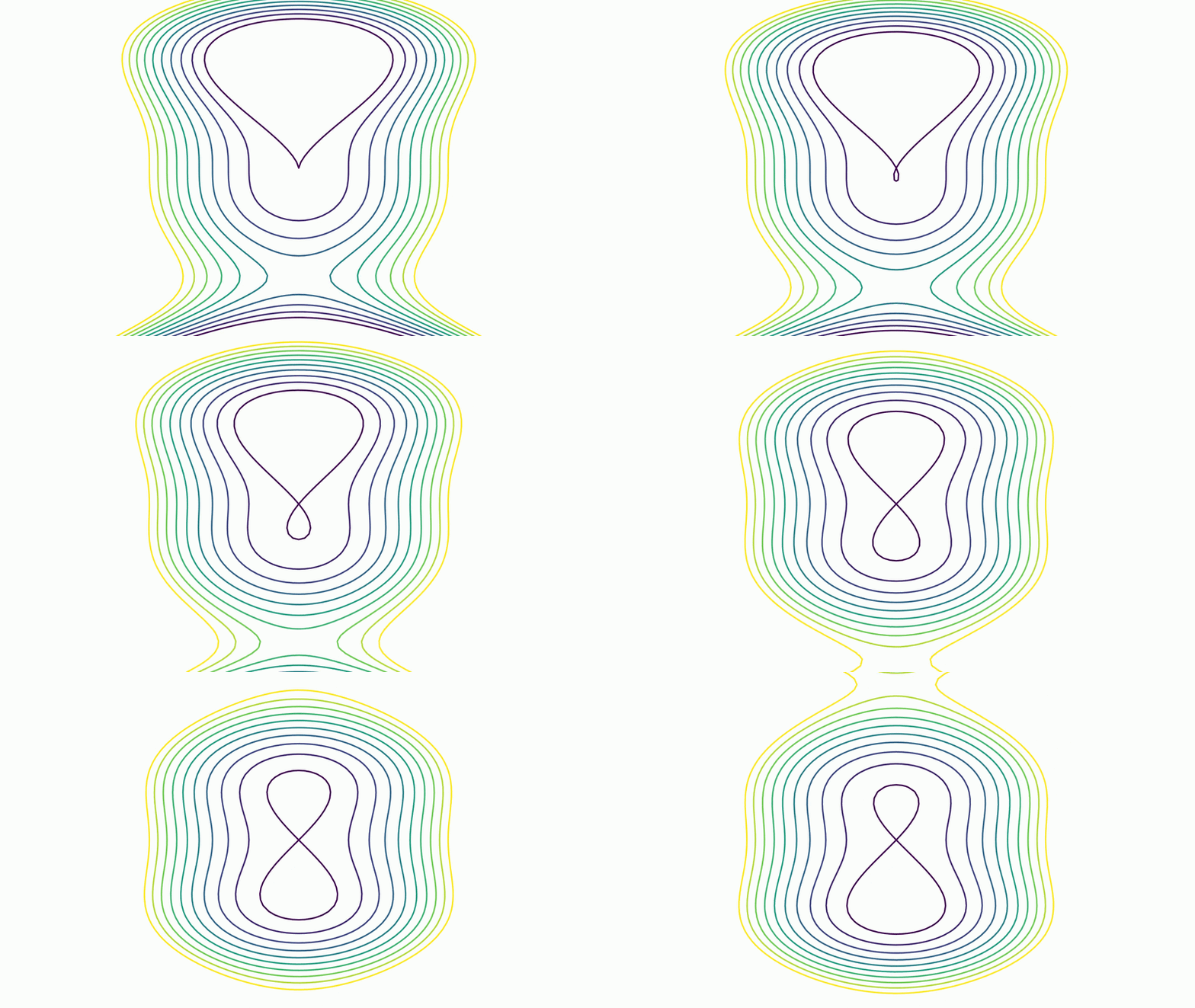
Here is the fun part, and it works the same for all three objects. If your field function takes an additional parameter, say t, that t becomes an animatable value. Animate it with the animScalar DSL command (it drives t from one value to another and recomputes the field every frame):
def cp = contourPlot(
    function: { x, y, t -> x*x - y*y*Math.sin(PI*y + t) },
    rect:     [-2, -2, 2, 2],
    cols: 100, rows: 100,
    levels:   linspace(0, 1, 10),
    colorScale: [["blue", 0], ["red", 1]]
)
animScalar(obj: cp, from: 0, to: 2, runtime: 3)   // t: 0 to 2 over 3 seconds
The same idea animates a density plot or a vector field. Feel free to try!
def dp = densityPlot(function: { x, y, t -> Math.sin(x + t) * y })
animScalar(obj: dp, from: 0, to: 2*PI, runtime: 4)

def vf = vectorField(function: { x, y, t -> Vec.to(Math.cos(t)*x, y) })
animScalar(obj: vf, from: 0, to: 2*PI, runtime: 4)
In plain Groovy:
animScalar(obj: cp, from: 0, to: 2, runtime: 3)is the DSL twin ofplay.scalar(3, 0, 2, cp).
Performance note: the field is sampled on a background thread when possible (the default). If your function relies on shared mutable state and isn't thread-safe, turn that off by adding parallel: false to the DSL block.
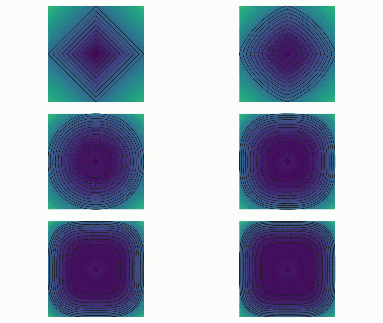
Of course you can animate several objects at the same time. Note in the following example that the contourPlot object has layer 1 to ensure is being drawn over the densityPlot object:
def f = { x, y, t -> Math.pow(Math.abs(x), t) + Math.pow(Math.abs(y), t) }
def cp = contourPlot(
    function: f,
    levels: [min: 0, max: 1.0, step: 0.1],
    rect: "centered", //Unit square centered at origin
    layer: 1
)
def dp = densityPlot(
    function: f,
    colorScale: ["viridis", 0, 3],
    rect: "centered",
    layer: 0
)

animScalar(
    obj: [cp, dp],
    from: 1, to: 4,
    runtime: 4
)
A value of your own: scalar
The t of a field is animatable because the field is a Parametric object, one that holds a number. You can create such a number on its own with scalar(...), and then everything else in the scene can follow it:
def t = scalar(0) // or scalar(value: 0), the same thing
A scalar is not drawn and is not a MathObject: it is a value other things read. What makes it useful is that animScalar moves it exactly like it moves the t of a field, so any drawing that depends on it moves too:
def t = scalar(0)
def P = point(at: [1, 0], style: [drawColor: "red", thickness: 40], addToScene: true)

// P follows the value on every frame
always(obj: P, dependsOn: t) { obj ->
    obj.moveTo(Math.cos(t.value), Math.sin(t.value))
}

animScalar(obj: t, from: 0, to: 2*PI, runtime: 4)
Read and write it with t.value (t.getValue() / t.setValue(v)); t.add(delta) and t.lerp(target, alpha) move it by hand. It can also feed a text through a link, as in the Dynamic text chapter:
def readOut = latex(text: r"$t = {#0}$", format: "0.00", stack: [screen: "upper_left"])
link(from: t, fromType: "value", to: readOut, toType: "arg0")
Showing the value: slider
A number moving out of sight is hard to follow, so slider(...) draws it: a track, a marker where the value falls, the ends of the range and the current value.
def a = scalar(0)
slider(value: a, from: 0, to: 1, label: r"$a$",
       stack: [screen: "lower_right", gaps: 0.2], addToScene: true)

animScalar(obj: a, to: 1, runtime: 4)     // the marker moves on its own
The track can run either way, and its length is up to you:
slider(value: a, orientation: "vertical", length: 3, from: -2, to: 2)
The rest of the parameters are about how much of it is drawn and how it looks: format (of the value and the ends), showValue, showEnds, gap, labelScale, and style / knobStyle / labelStyle for the track, the marker and the labels. A plain number in value gives a fixed, decorative slider.
The call returns the track, and the pieces are inside it:
def sl = slider(value: a, from: 0, to: 1)
def knob = sl.getInternalObject("knob")    // also "value", "name", "min", "max"
Since every piece is placed relative to the track on each frame, moving, stacking or transforming the returned object drags the whole slider along, and the marker keeps following the value.
Building lists of levels: linspace and arange
Typing out twenty contour levels by hand is nobody's idea of fun. JMathAnim ships two Python/NumPy-style helpers, available directly in any script (no prefix needed), that build the list for you:
// 21 evenly spaced levels between -1 and 1, both endpoints included
def levels = linspace(-1, 1, 21)

// From -1 up to (but not including) 1, in steps of 0.1
def levels = arange(-1, 1, 0.1)
You can drop either one straight into the levels: parameter:
contourPlot(
    function: { x, y -> Math.sin(x)*Math.sin(x) + Math.cos(x)*Math.cos(y) },
    rect:     [-3, 3, -3, 3],
    levels:   linspace(-1, 1, 21)
)
The one gotcha: arange(start, stop, step) treats stop as exclusive (just like NumPy), so arange(-1, 1, 0.1) stops at 0.9 and misses 1.0. If you need the endpoint, either push stop slightly past it (arange(-1, 1 + 0.05, 0.1)) or use linspace, which always includes both ends by design and is usually the friendlier choice.