Basic Objects
This chapter covers the fundamental building blocks of JMathAnim animations. All drawable objects inherit from the MathObject class (or implement the Drawable interface), which provides common methods for transformations like scale, rotate, and shift.
How to read this chapter: it's a catalog, not a novel. Read the Vec, Point, Shape and LatexMathObject sections first (you will use them in every single animation), skim the rest, and come back when you need an arrow or a grid. And remember: almost every object here has a ready-made snippet in the editor (press Alt+S, type the first letters of the object name, and the code writes itself). If a snippet inserts a DSL block, Ctrl+Space inside it shows all the available parameters.
Table of Contents
- The Vec Class
- The Point Class
- The Shape Class
- The LatexMathObject Class
- The Line Class
- The Axes Class
- The CartesianGrid Class
- Boards
- Importing Images
- The MathObjectGroup Class
- Compound Objects
- The Rect Class
The Vec Class
The Vec class represents a 2D vector (with an additional z-coordinate for future 3D support). It's not at object can be added to scene or drawn, but it's the fundamental class for representing coordinates in the math view and defining parameters in most objects.
Creating Vectors
def v = Vec.to(4, 5)        // Creates vector (4, 5)
def w = Vec.to(2, -1)       // Creates vector (2, -1)
def origin = Vec.origin()   // Creates vector (0, 0)
def random = Vec.random()   // Creates a vector in a random screen location
Accessing Components
def x = v.x                 // Get x-coordinate
def y = v.y                 // Get y-coordinate
def norm = v.norm()         // Get Euclidean norm (length)
Vector Operations
JMathAnim provides two styles of vector operations:
-
Immutable operations - Return a new vector, leaving the original unchanged:
def sum = v.add(w) // Returns v + w (new vector) def scaled = v.copy().scale(3) // Returns 3v (new vector, v unchanged) def diff = v.to(w) // Returns w - v (new vector) -
In-place operations - Modify the original vector:
v.scale(3)                  // Multiplies v by 3 (modifies v)
v.shift(w)                  // Adds w to v (modifies v)
v.rotate(45 * DEGREES)      // Rotates v by 45° (modifies v)
Additional Methods
def dot = v.dot(w)          // Dot product of v and w
def angle = v.getAngle()    // Angle in radians (0 to 2π)
Note: The DEGREES constant converts degrees to radians. Use it for all angle operations: angle * DEGREES.
The Point Class
The Point class is the most basic MathObject, representing a single point in space. The main difference between a Point and a Vec
class is that the Vec is a lightweight object to hold coordinates, while Point is a MathObject that can be drawn on screen.
Creating Points
def p = Point.at(1, 1)      // Point at coordinates (1, 1)
def q = Point.at(v)         //Point at coordinates given by vector v
def r = Point.origin()      // Point at (0, 0)
def s = Point.random()      // Point at random screen location
Accessing Coordinates
Points contain a Vec object storing their position:
def v = p.getVec()          // Get position vector
def x = p.getVec().x        // Get x-coordinate
def d = p.norm()            // Distance from origin
def AB = A.to(B)            // Vector from point A to point B
Point Styles
Points can be displayed in various styles using the DotStyle enum:
def A = Point.at(-1.75, 0).dotStyle(DotStyle.CIRCLE)
def B = Point.at(-1.25, 0).dotStyle(DotStyle.CROSS)
def C = Point.at(-0.75, 0).dotStyle(DotStyle.PLUS)
def D = Point.at(-0.25, 0).dotStyle(DotStyle.RING)
def E = Point.at(0.25, 0).dotStyle(DotStyle.TRIANGLE_UP_HOLLOW)
def F = Point.at(0.75, 0).dotStyle(DotStyle.TRIANGLE_DOWN_HOLLOW)
def G = Point.at(1.25, 0).dotStyle(DotStyle.TRIANGLE_UP_FILLED)
def H = Point.at(1.75, 0).dotStyle(DotStyle.TRIANGLE_DOWN_FILLED)

scene.add(A, B, C, D, E, F, G, H)

// Add reference axis
scene.add(
    Line.XAxis()
        .thickness(2)
        .drawColor("gray")
        .layer(-1)  // Draw behind points
)

I showed you this 'manual code', which describes each point individually, to demonstrate the various style names. Of course, a similar image could also be created using loops:
def x0=-1.75 //Initial value 0f x0
for (style in DotStyle) { //Iterate over DotStyle values
    def P=Point.at(x0,0).dotStyle(style)
    scene.add(P)
    x0+=0.5 //Add 0.5 to x0
}

//The axis code is the same...
Note: Points require higher thickness values (typically 20-40) to be clearly visible, as the thickness represents the point's diameter.
You can also create it using the DSL:
def A = point(at: [-1.75, 0], style: [dotStyle: "cross", color: "blue", thickness: 30])
The Shape Class
The Shape class is one of the most important classes in JMathAnim. It represents curves (closed or open) and provides extensive functionality for creating and manipulating 2D shapes.
Basic Shape Constructors
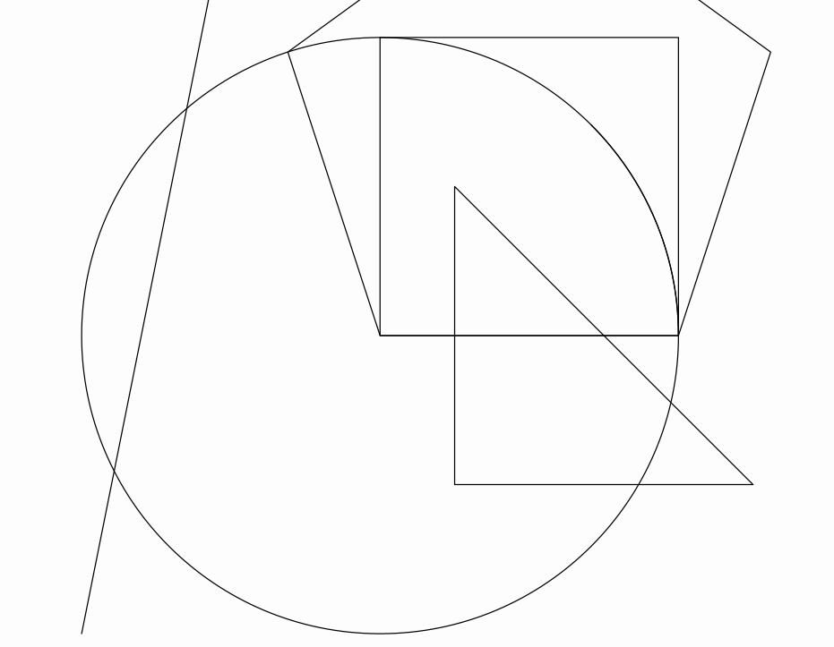
JMathAnim provides convenient static methods for common shapes:
// Circle with radius 1, centered at origin
def circ = Shape.circle()

// Unit square with lower-left corner at origin
def sq = Shape.square()

// Regular pentagon with first two vertices at (0,0) and (1,0)
def reg = Shape.regularPolygon(5)

// Triangle from specified vertices
// Accepts Vec, Point, or any Coordinates object
def poly = Shape.polygon(
    Vec.to(0.25, -0.5),
    Vec.to(1.25, -0.5),
    Vec.to(0.25, 0.5)
)

// Axis-aligned rectangle
// Parameters: lower-left corner, upper-right corner
def rect = Shape.rectangle(Vec.to(1, 2), Vec.to(3, 5))

// Line segment between two points
def seg = Shape.segment(Vec.to(-1, -1), Vec.to(-0.5, 1.5))

// Circular arc
// Parameters: arc length in radians
def arc = Shape.arc(PI / 4)

scene.add(circ, sq, reg, poly, rect, seg, arc)
Creating Shapes with LOGO Commands
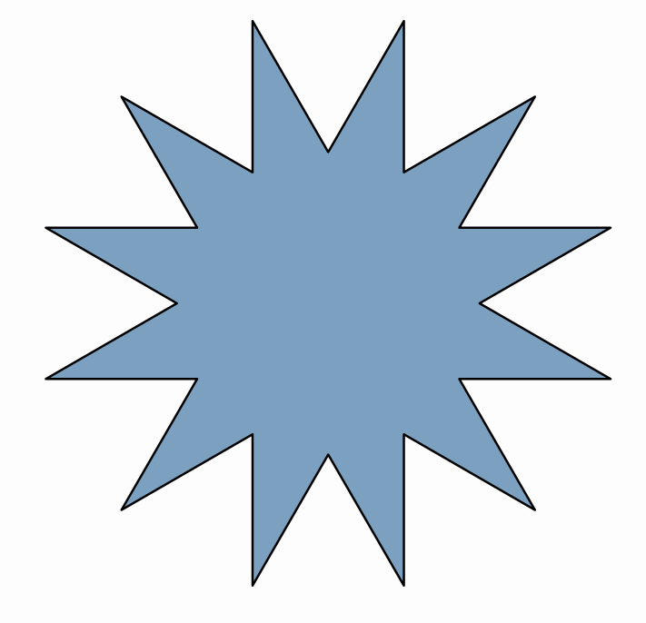
Shapes can also be created using LOGO turtle graphics commands, which is useful for complex or iterative patterns:
// CLO (or CLOSE) is a non-standard command to close the path
def logoCmd = "REPEAT 12 [FD .5 RT 150 FD .5 LT 120] CLO"
def logoShape = Shape.logo(logoCmd)

scene.add(
    logoShape
        .center()
        .style("solidblue")
)
Supported LOGO Commands
| Command | Aliases | Description |
|---|---|---|
FORWARD n |
FD n |
Move forward n units |
BACKWARD n |
BK n |
Move backward n units |
RIGHT angle |
RT angle |
Turn right by angle degrees |
LEFT angle |
LT angle |
Turn left by angle degrees |
REPEAT n [commands] |
Execute commands n times | |
PENUP |
PU |
Lift pen (move without drawing) |
PENDOWN |
PD |
Lower pen (resume drawing) |
LARC / RARC angle radius |
Left/Right arc (JMathAnim extension) | |
CLOSE |
CLO |
Close the path (JMathAnim extension) |
Commands are case-insensitive. Full reference available at Logo Commands Reference.
Storing and Restoring Shapes with SVG Path Commands
Any Shape can be encoded as a string of SVG path commands, the same syntax used by the d attribute of a path element in a SVG file. This is the most compact way to keep a Shape in a text file, or even in a plain String inside the code, and rebuild it later:
def heart = Shape.logo("REPEAT 12 [FD .5 RT 150 FD .5 LT 120] CLO")

// Geometry as a String, with 6 decimals by default
def code = heart.toSVGPath()      // "M0 0L.5 0C..."

// And back to a Shape
def restored = Shape.fromSVGPath(code)
Only the geometry travels in the string, no style at all. toSVGPath(decimals) sets the precision of the coordinates, which is where most of the size comes from: toSVGPath(3) is usually enough for a drawing and gives a much shorter string. Straight segments are stored as L commands, so they carry no control points.
Since the syntax is standard, the string can be pasted into a SVG file, and a path copied from a vector editor such as Inkscape can be read directly:
def star = Shape.fromSVGPath("M50 5L61 40H98L68 62L79 97L50 75L21 97L32 62L2 40H39Z")
scene.add(star.center().height(2))
The DSL form is shape(type: "svgpath", path: "...").
Compressed Paths
For a detailed shape, with hundreds of points, the commands string gets long. toCompressedPath() deflates it and encodes the result in Base64, which typically divides the size by 3 to 5:
def code = heart.toCompressedPath()   // "JMA1:eJx1kMFqwzAQ..."
def restored = Shape.fromSVGPath(code)
The compressed string is tagged with a JMA1: prefix, so Shape.fromSVGPath (and the svgpath DSL type) tells the two forms apart and reads either one. It only holds letters, digits and the characters -, _ and :, so it needs no escaping and can be stored in a String, a properties file, a YAML file or a URL. Whitespace inside it is ignored, and it can be split over several lines.
toCompressedPath(decimals) sets the precision, exactly as toSVGPath(decimals) does.
Storing the Style Too
The methods above keep only the geometry. toStyledPath() stores the style as well, as a list of properties in front of the path commands:
def s = Shape.circle().thickness(4).drawColor("maroon").fillColor("deeppink1")

def code = s.toStyledPath()
// "drawColor=#800000FF;fillColor=#FF1493FF;thickness=4;dashStyle=SOLID;...|M1 0C1 .5523..."

def restored = Shape.fromSVGPath(code)   // same drawing, same style
The property names are the ones used in the style maps of the DSL and in the styles of the config files: drawColor, fillColor, thickness, dashStyle, lineCap, lineJoin, strokeType, layer, thicknessTracksZoom and thicknessTracksScale. Only the properties actually set are written, and colors are stored as #RRGGBBAA. A gradient or an image pattern does not fit in a single value, so it is skipped with a warning and only the rest of the style travels.
toCompressedStyledPath() is the compressed version, and Shape.fromSVGPath reads any of the four codes, telling them apart by the JMA1: prefix and by the | separator:
| Method | Style | Compressed |
|---|---|---|
toSVGPath() |
no | no |
toCompressedPath() |
no | yes |
toStyledPath() |
yes | no |
toCompressedStyledPath() |
yes | yes |
When the code has no style, the default one is applied. In the DSL, shape(type: "svgpath", path: code, style: [...]) applies the stored style first, so the style parameter still has the last word.
DSL Syntax
Since core version 1.3.5, the script interpreter admits several commands defined in DSL syntax to build objects in a more accessible way:
def s = shape(
    type: "circle",
    segments: 30,
    style:[thickness: 30, drawcolor: 'maroon',fillcolor: 'deeppink1'],
    addToScene: true
)
Is equivalent to
def s=Shape.circle(30).thickness(30).drawColor('maroon').fillColor('deeppink1')
scene.add(s)
The gui editor has built autocomplete for most DSL commands as well as a snippet sidebar to speed code generation. You can see a cheatsheet of DSL commands here
Working with Shape Paths
Each Shape contains a JMPath object that manages its path. Points can be accessed using zero-based circular indexing:
def pentagon = Shape.regularPolygon(5) //Has points with indices 0, 1, 2, 3, 4

def p0 = pentagon.getPoint(0)    // First vertex
def p1 = pentagon.getPoint(1)    // Second vertex
def p5 = pentagon.getPoint(5)    // Wraps around to first vertex (same as p0)
Important: Shape points use circular array indexing, so getPoint(n) and getPoint(n + vertexCount) return the same point.
Shape Centers
Shapes provide two methods for finding their center:
def bbox_center = shape.getCenter()     // Center of bounding box (returns a Vec object)
def geometric_center = shape.getCentroid()  // Average of all vertices
Note: For regular polygons, .getCentroid() returns the true geometric center, while .getCenter() returns the center of the bounding box, which may differ for rotated shapes.
Measuring a shape
Every shape answers for the area it encloses and the length of its path, which is the perimeter when the path is closed:
def a = pentagon.area       // area enclosed, signed by the orientation of the path
def per = pentagon.length   // length of the path: the perimeter, as it is closed
def arcLength = arc.length  // an open path simply gives its length
Both are properties, so they read as shown, without get and parentheses.
The LatexMathObject Class
The LatexMathObject class renders mathematical expressions using LaTeX, allowing you to display formulas and text with professional typesetting.
Creating LaTeX Objects
def text = LatexMathObject.make("This is a \\LaTeX equation \$e^{i\\pi}+1=0\$")
scene.add(text)

You can also create it using the DSL, with the latex(...) command (a plain, non-LaTeX text object is available through text(...)):
def text = latex(text: r"This is a \LaTeX equation $e^{i\pi}+1=0$")
Handling Special Characters
LaTeX uses $ and \ as special characters. In Groovy, these must be escaped:
// INCORRECT - Groovy will interpret $ and \ as escape sequences
LatexMathObject.make("$e^{i\pi}+1=0$")  // ERROR!

// CORRECT - Escape the special characters
LatexMathObject.make("\$e^{i\\pi}+1=0\$")  // Works!

// BETTER - Use raw strings (prefix with 'r')
LatexMathObject.make(r"$e^{i\pi}+1=0$")  // Easiest!
Tip: Raw strings (prefixed with r) ignore escape sequences. Use either single or double quotes:
LatexMathObject.make(r"$e^{i\pi}+1=0$")  // Both work
LatexMathObject.make(r'$e^{i\pi}+1=0$')  // identically
Let the editor do it: if writing LaTeX by hand is not your idea of fun, place the cursor inside the string and open the LaTeX Editor (
Tools -> LaTeX Editor..., orCtrl+Shift+L). You get a live preview while you type, and theInsert Codebutton writes the (correctly escaped) string back into your script for you.
Also, you can use triple quotes to enable multiline strings:
def text = LatexMathObject.make(r'''
$$
ax^2+bx+c=0
$$
''')
scene.add(text)
Compilation Modes
JMathAnim offers two LaTeX compilation methods:
-
Default (JLaTeXMath) - Fast, built-in renderer for most formulas:
def formula = LatexMathObject.make(r'$e^{i\pi}+1=0$') -
External LaTeX - Uses system LaTeX for advanced features:
def formula = LatexMathObject.make(
    r'$e^{i\pi}+1=0$',
    CompileMode.CompileFile
)
The external compiler:
- Requires a LaTeX distribution installed on your system
- Compiles to
.dvi, converts to.svg, imports asMultiShapeObject - Caches
.svgfiles for reuse in subsequent runs - Supports commands not available in JLaTeXMath (e.g.,
\begin{verbatim}), but in most cases JLaTexMath will be enough.
Recommendation: Use the default mode (JLaTeXMath) unless you need advanced LaTeX features.
The Line Class
The Line class represents infinite mathematical lines. In practice, it draws the visible portion within the current view.
Creating Lines
def A = Point.at(1, 1)
def B = Point.at(0, 1)
def v = Vec.to(1, 0.2)

// Line through points A and B
def line1 = Line.make(A, B)
    .drawColor("red")
    .thickness(20)

// Line through A in direction v
def line2 = Line.make(A, A.add(v))
    .drawColor("blue")
    .thickness(10)

// Predefined axes
def line3 = Line.XAxis().drawColor("darkorange")        // y = 0
def line4 = Line.YAxis().drawColor("darkmagenta")       // x = 0
def line5 = Line.XYBisector().drawColor("darkgreen")    // y = x

scene.add(line1, line2, line3, line4, line5)
play.shift(5, -1, -1.5, A)  // Animate point A
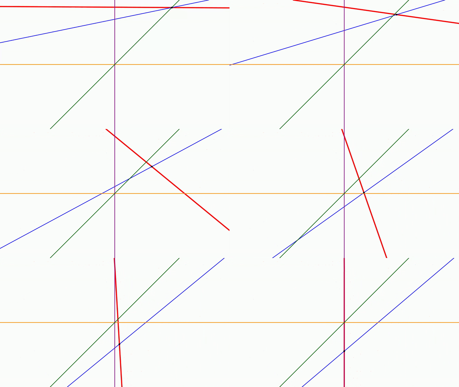
Note: Lines use direction vectors only at construction time. Moving a point after creating the line won't update the line's direction (unlike constraints, which are covered in advanced topics).
The Ray Class
Similar to Line, the Ray class represents half-infinite rays with syntax identical to Line constructors.
The Axes Class
The Axes class creates Cartesian coordinate axes with customizable ticks and labels. It's essentially a container managing multiple Line, Shape, and LatexMathObject instances.
Creating Axes
def axes = Axes.make()

// Add primary ticks
axes.generatePrimaryXTicks(-2, 2, 0.5)  // x: -2, -1.5, -1, ..., 2
axes.generatePrimaryYTicks(-2, 2, 0.5)  // y: -2, -1.5, -1, ..., 2

// Add custom ticks
axes.addXTicksLegend(0.75, TickType.PRIMARY)  // Tick at x = 0.75
axes.addYTicksLegend(r"$\pi/4$", PI / 4, TickType.PRIMARY)  // Custom label

scene.add(
    axes,
    Shape.circle()
        .scale(0.5)
        .drawColor("darkblue")
)
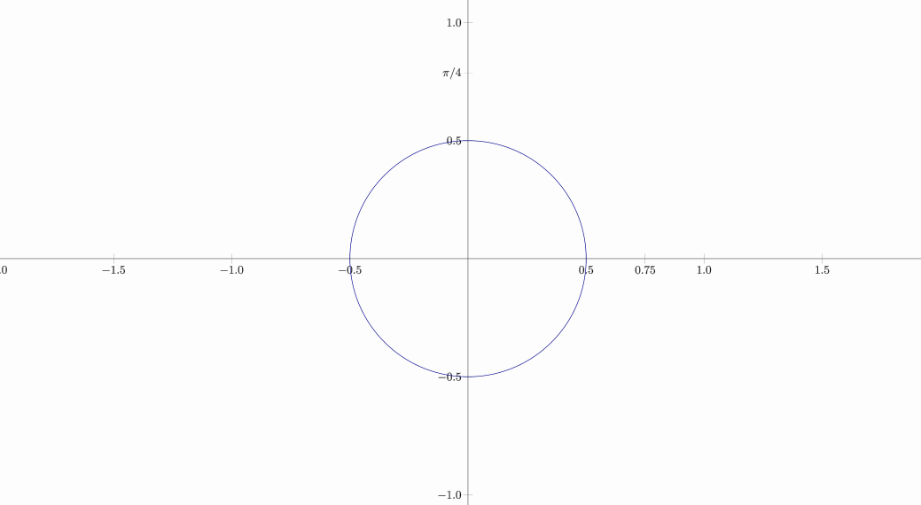
Note: By default, axes are created without ticks. Use generatePrimaryXTicks and generatePrimaryYTicks to add them.
Using the DSL format is even easier:
def axes = axes(
    range:[-2, 2],
    secondary: [maxwidth:0],
    ticksx: [0.75],
    ticksy: [[at: PI/4, label: '$\\pi/4$', type:"sec"]]
)
The CartesianGrid Class
Creates a grid with primary and secondary divisions, useful for reference and measurements.
// Grid centered at origin with subdivisions
def grid = CartesianGrid.make(
    0, 0,       // Center point (usually origin)
    2,          // Horizontal subdivisions for secondary grid
    2           // Vertical subdivisions for secondary grid
)

scene.add(
    grid,
    Shape.circle()
        .drawColor("blue")
        .fillColor("blue")
        .fillAlpha(0.5)
)
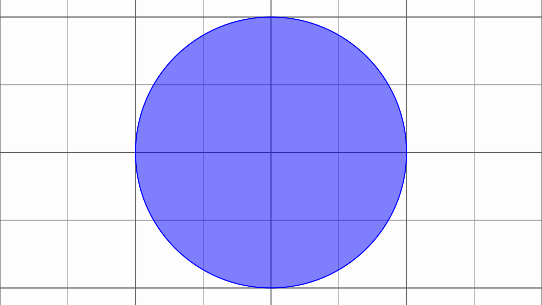
Styling: Grids use the gridPrimaryDefault and gridSecondaryDefault styles defined in your config files. See the Styling chapter for customization details.
You can also use the DSL version
def grid = grid(
    center:[0, 0], //Optional
    divisions: 2 //equivalent to divisions:[2,2]
)
Looking for arrows, connectors or delimiters? Those objects (which point at, join or bracket other objects) now live in their own chapter: Arrows, connectors and delimiters. Function graphs and other calculus-flavored objects are in Calculus objects.
Boards
While a grid extends over the whole view, a board is a bounded rectangle divided into cells: the chessboard, a table, the cells of a game. The board(...) DSL builds it as a compound of Shapes, so it enters the scene, moves and is styled as a single object.
def b = board(width: 4, columns: 8) //4x4 chessboard, 8x8 cells, centered at the origin
The size is given with width and height (which defaults to width, so a single number gives a square board) around a center, or with rect for the whole region at once. The number of cells is columns and rows (which defaults to columns), or divisions as a shorthand for both.
def b1 = board(width: 6, height: 3, columns: 4, rows: 2)
def b2 = board(rect: [-2, -1, 2, 1], divisions: [8, 4])
def b3 = board(divisions: 3)          //unit 3x3 board: the tic-tac-toe grid
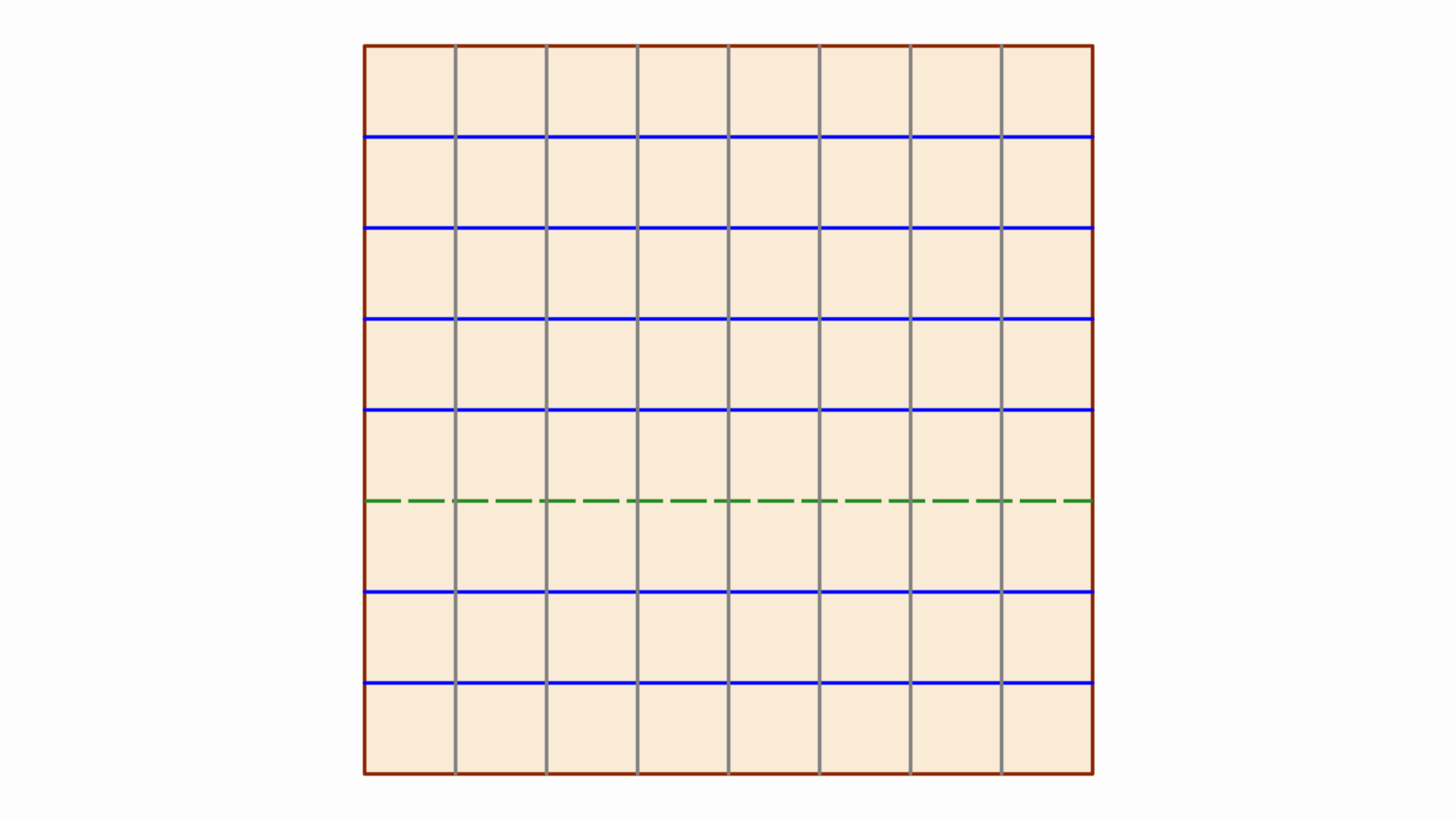
Every piece of the compound has a name of its own. The outer border is a single closed rectangle named border, and the inner lines are segments: v1 to v<columns-1> for the vertical ones, left to right, and h1 to h<rows-1> for the horizontal ones, bottom to top. So an 8-column board has the border plus 7 inner vertical lines. That gives each piece to parts: and to the subscript operator:
def b = board(width: 4, columns: 8,
              style: [thickness: 2],
              parts: ["border": [color: "red", thickness: 5], "h*": [color: "gray"]])
b["v4"].thickness(6)                  //the middle line, thicker
The glob selectors make it easy to give a different color to each family of pieces:
def b = board(width: 2, columns: 8, rows: 8,
      style: [thickness: 10],
      parts: [
          "border": [drawcolor: "orangered4",
              fillColor: 'antiquewhite'],
          "v*": [color: "gray",//style for all vertical lines
              layer: 1,
              thickness: 10],
          "h*": [color: "blue"],//style for all horizontal lines
          "h3": [dashstyle: "dashed",//syle for third only
              drawcolor: 'forestgreen']
      ]
)
scene.add(b)
Importing Images
JMathAnim supports both bitmap and vector images. Images are loaded from the resources/images/ folder by default (configurable in styling settings).
The image DSL
One call covers both kinds: the importer is chosen from the file extension (.svg means vector, anything else bitmap) and can be forced with type:.
def img = image(file: "euler.jpg", transform: [height: 2, center: true])
def svg = image(file: "knuth.svg", transform: [height: 2], addToScene: true)

appear(obj: img, type: "movein", from: "left", runtime: 2)
Sizing goes through the usual transform: map (height, width, scale), and stack: places the image like any other object. Two parameters are specific to images:
preserveRatio: truekeeps the aspect ratio of a bitmap when it is resized.adjustTo: [A, B]puts the lower left and lower right corners of the image on those two points, shifting, rotating and scaling it in one go. It replaces any previous placement, so it is applied beforetransformandstack.
image(file: "photo.jpg", adjustTo: [[-1, -1], [1, -1]])
image(file: "!C:/tmp/absolute.png")     // the "!" prefix takes an absolute path
Images take no label: (they are not label-locatable): build a separate latex(...) or text(...) and stack it to the image instead.
Bitmap Images
Import any bitmap format supported by JavaFX (PNG, JPG, etc.):
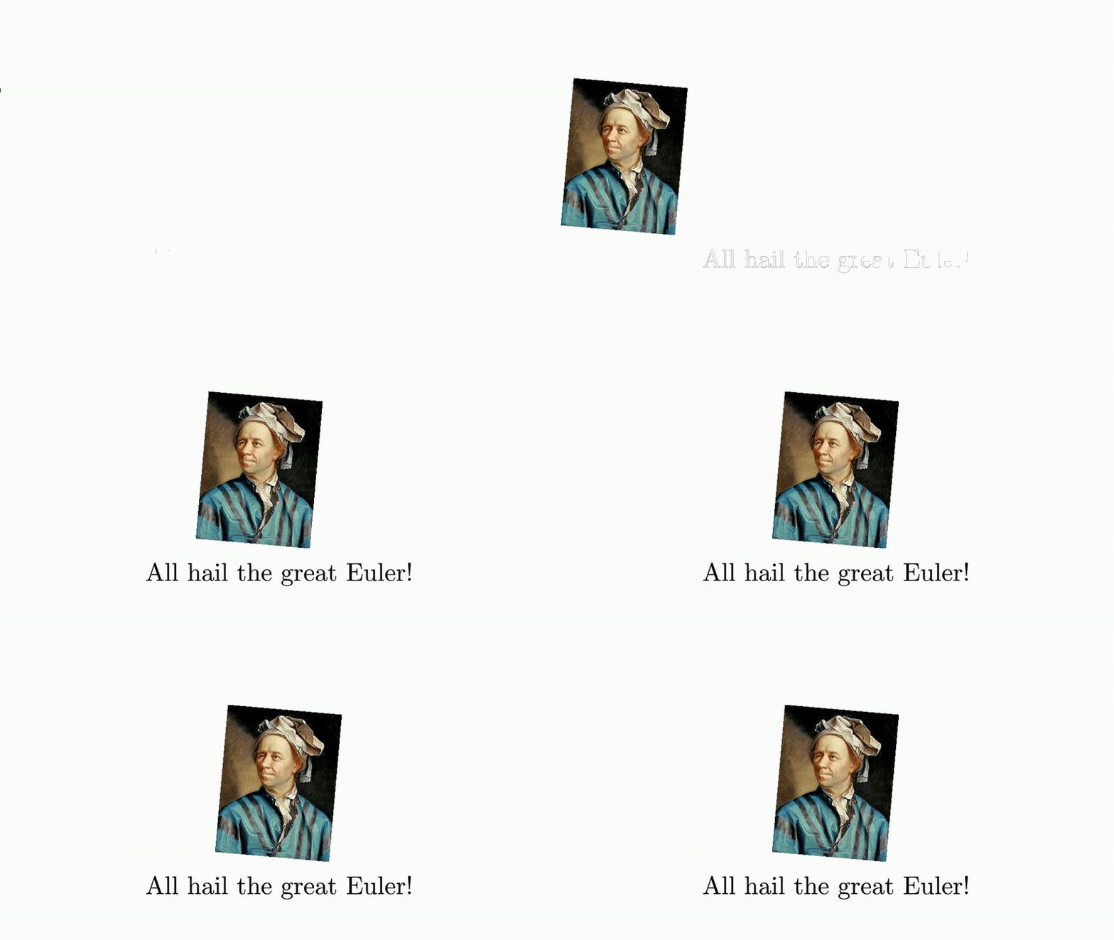
def img = image(
      file: "euler.jpg",
      transform: [height: 1.5, center: true, rotate: -5 * DEGREES],
)

def text = latex(
      text: "All hail the great Euler!",
      stack: [to: img, gaps: .1, destinyanchor: "lower"]
)
play {
    appear(
          runtime: 2,
          type: "movein", from: "left",
          obj: img
    )
    appear(
          runtime: 2,
          type: "showcreation",
          obj: text
    )
}
animWait(3)
SVG Images
Import and animate SVG vector graphics:
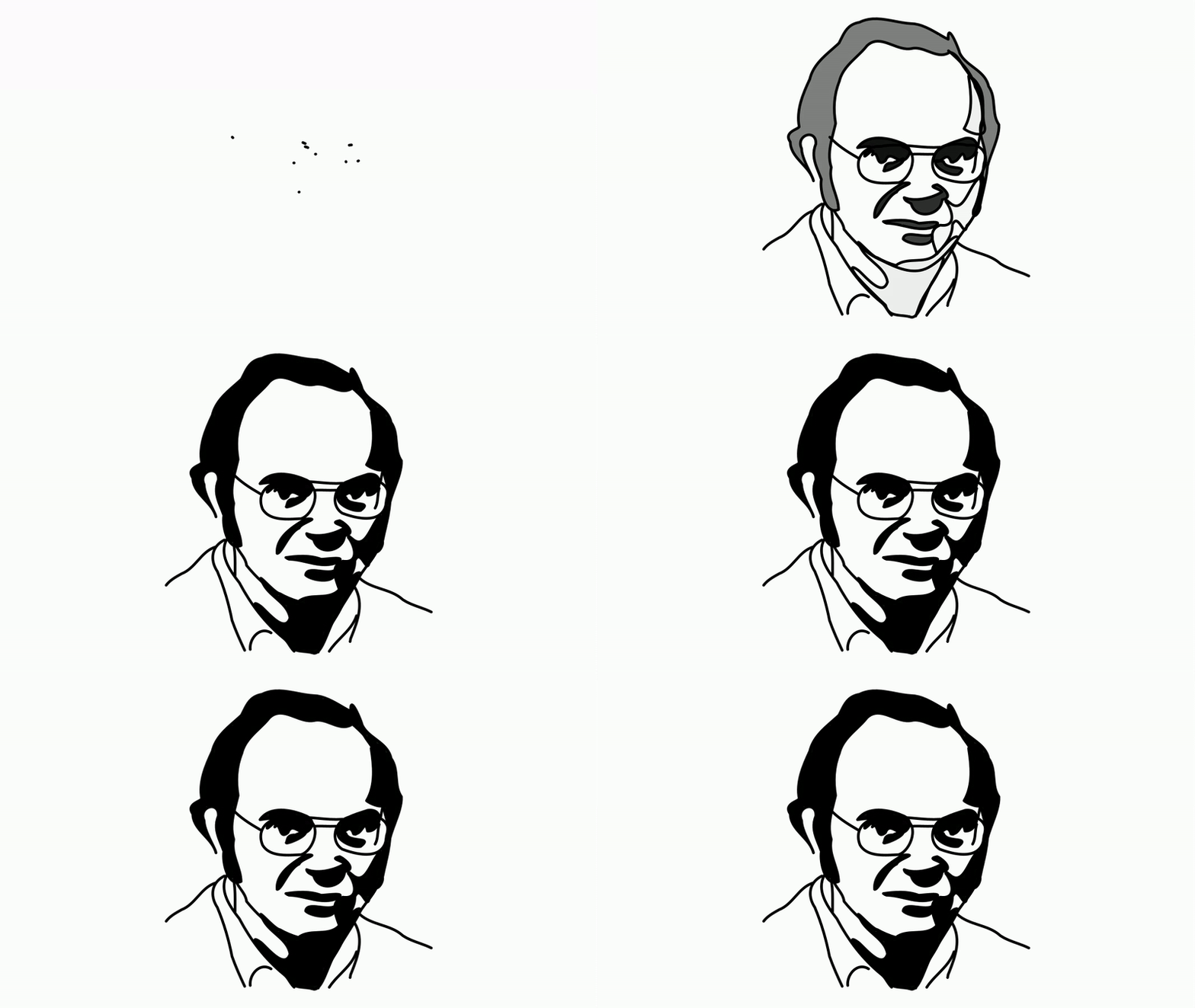
def svg=image(
    file: "donaldKnuth.svg",
    transform: [height: 2, center: true]
)
appear(
    runtime: 1,
    type: "showcreation",
    obj: svg
)
animWait(2)
File Location: Place SVG files in <project_root>/resources/images/
SVG Import Details:
- Creates a MultiShape object containing multiple Shape instances
- Each SVG element becomes a separate Shape with a JMPath
- Supports standard transformations and animations
- Limitation: Some elements (e.g., gradients) may not import with 100% accuracy
The MathObjectGroup Class
MathObjectGroup manages collections of MathObject instances as a single entity, enabling batch operations and layouts.
Creating Groups
def square = Shape.square()
def triangle = Shape.regularPolygon(3)
def circle = Shape.circle()

def group = MathObjectGroup.make(square, triangle, circle)
Group Operations
Groups support all standard MathObject operations:
group.shift(1, 1)              // Move entire group
group.rotate(45 * DEGREES)      // Rotate all members
group.scale(2)                  // Scale all members
group.setFillColor("cadetblue") // Apply to all members
Aligning the elements
align(...) moves every element of the group against the bounding box of the group itself, so all of them end up sharing the same side or centerline. It takes an AlignType, or a String naming one: upper, lower, left, right, hcenter, vcenter or baseline.
group.align("left")                     // every element to the left side of the group
group.align(AlignType.VCENTER)          // all of them centered vertically
The same thing is a key of the group(...) block, applied after the layout, and of apply(...), where several objects are aligned among themselves and a single group has its elements aligned:
def g = group(obj: [a, b, c], layout: "lower", align: "left")
apply(obj: g, align: "hcenter")
apply(obj: [a, b, c], align: "upper")
baseline aligns the baselines of the texts with each other, the same thing alignBaselines() does. Elements that are empty are left where they are.
Adding Groups to Scene
Adding a group is equivalent to adding all its members:
scene.add(group) // Same as: scene.add(square, triangle, circle)
Note: The MathObjectGroup is a logical group. It does not represent an object by itself and cannot be added to the scene. It is just a way to tell the interpreter "work with this group of objects".
Why Use Groups?
Groups excel at: - Batch transformations: Transform multiple objects together - Layout management: Arrange objects automatically (see TransformingObjects chapter) - Animation coordination: Animate multiple objects as one unit
Example using layouts:
def group = MathObjectGroup.make(square, triangle, circle)
group.setLayout(LayoutType.LOWER, 0.1, 0.1)  // Arrange vertically
scene.add(group) //The same as scene.add(square, triangle, circle)
Naming the elements
The group(...) DSL block takes a Map in obj: instead of a list, and stores each key in the dictionary of the group. The elements keep their order, and each one can be reached, styled or animated by its name instead of by its index:
def g = group(obj: [body: shape(type: "circle"),
                    head: shape(type: "square")],
              layout: "upper", gap: 0.1)

g["head"].color("red")                       // the element, by name
apply(obj: g, parts: [head: [fillColor: "gold"]])
g.parts()                                    // name -> element
The same names work in every parts: map (see the Styling chapter), so a group built this way behaves like the built-in composite objects.
Compound Objects
A group is a logical container. When you need the opposite, an object of your own made of several pieces that behaves as one thing, the compound(...) block builds a CompoundMathObject:
def balance = compound(
    obj: [base: shape(type: "square"),
          arm : shape(type: "segment", from: [-2, 1], to: [2, 1]),
          panL: shape(type: "polygon", points: [[-2,1],[-1.2,1],[-1.35,.65],[-1.85,.65]]),
          panR: shape(type: "polygon", points: [[1.2,1],[2,1],[1.85,.65],[1.35,.65]])],
    style: [color: "gray"],
    parts: [panL: [fillColor: "red"], "pan*": [thickness: 3]],
    addToScene: true)
The parameters are the same ones group(...) takes (obj, copies and number, layout, gap, homogeneize, align, plus the common style, parts, transform, stack...). What changes is where the pieces live:
group(...) |
compound(...) |
|
|---|---|---|
scene.add(...) |
adds the members, one by one | adds the compound itself |
| Drawing | each member draws itself | the compound draws its pieces |
| Removing it | removes the members | removes the whole object |
| Its pieces | scene objects of their own | internal to the compound |
So group is the tool to operate in bulk on objects that are their own citizens of the scene, and compound is the tool to build a new object out of parts. Reaching the pieces works the same in both:
balance["arm"].color("black")                     // a piece, by its name
balance["panL", "panR"].color("red")              // several at once: a MathObjectGroup
apply(obj: balance, parts: [base: [color: "brown"]])
animRotate(obj: balance, angle: 7 * DEGREES, center: [0, 1])   // the whole object moves as one
A subscript returns the piece when the selector matches one and a group with all of them when it matches several (balance["pan*"], balance["panL,panR"]), so a selector never silently drops matches. That group is logical: the pieces stay inside the compound, which is still the one drawing them.
The pieces are written in drawing order, so panL above is drawn over base. Their layer orders them among themselves only; the layer of the compound is what places it among the objects of the scene. Note that compound(layer: n) also flattens the layers of the pieces, so per-piece layers are set afterwards:
balance.layer(2)                 // the whole object, over the layer-1 ones
balance["arm"].layer(1)          // and inside it, the arm over the rest
Compounds that do something
A compound can derive the position of its pieces from a few named values instead of being placed once and for all. state: declares them and rebuild: says where the pieces go:
def box = compound(
    obj:   [bottom: shape(type: "rectangle", rect: [-1, -.5, 1, -.4]),
            left:   shape(type: "rectangle", rect: [-1, -.5, -.9, .5]),
            right:  shape(type: "rectangle", rect: [.9, -.5, 1, .5]),
            lid:    shape(type: "rectangle", rect: [-1, .4, 1, .5])],
    state: [aperture: 0],                     // 0 closed, 1 open
    rebuild: { b ->
        b["lid"].rotate(b["left"].boundingBox.upperLeft,
                        125*DEGREES * b.delta("aperture"))
    })

animState(obj: box, to: [aperture: 1], runtime: 1.5)   // and the box opens
The value is what gets animated; the geometry follows. That is what makes the opening interruptible (closing halfway continues from where it is instead of jumping) and consistent with animations that save and restore states.
Inside rebuild: there are three readings of a value: b.state("n") the current one, b.previousState("n") the one the geometry on screen was built from, and b.delta("n") the difference. The difference is what an incremental rebuild uses: turning a piece by it lands the piece exactly where the value asks for, however many frames it took to get there. rebuild: runs once at the start and then only when a value has really changed, so a compound nobody touched costs nothing per frame.
Two more ways in:
apply(obj: box, state: [aperture: 1])     // set it without animating
box.state("aperture")                     // read it
Note that the pieces and the values live in different namespaces: box["lid"] is a piece, box.state("aperture") is a value.
For an object with methods of its own (box.openBox(1.5), box.isOpen()) the closure is not enough and you need a class: subclass StatefulCompound, declare the values in the constructor and implement rebuild(). The same apply(state:) and animState(...) work on it, so the two ways are the same thing with and without methods.
The chapter on compound objects builds one of these step by step.
The Rect Class
The Rect class represents axis-aligned bounding boxes. While not directly drawable, it's essential for positioning and collision detection or understanding how stacking and positioning works.
Getting Bounding Boxes
Every MathObject (and anything implementing Boxable) has a bounding box:
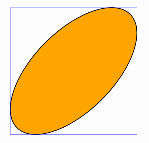
def ellipse = Shape.circle()
    .scale(1, 0.5)
    .rotate(45 * DEGREES)
    .style("solidorange")

def bbox = ellipse.getBoundingBox()  // Returns Rect
def rect = Shape.rectangle(bbox).drawColor("blue")

scene.add(ellipse, rect)
Rect Properties and Methods
// Corner coordinates
def xMin = bbox.xmin     // Left edge
def xMax = bbox.xmax     // Right edge
def yMin = bbox.ymin     // Bottom edge
def yMax = bbox.ymax     // Top edge

// Dimensions
def width = bbox.getWidth()  //...or bbox.width
def height = bbox.getHeight() //...or bbox.height

// Corner points
def center = bbox.getCenter() //or bbox.center
def upperLeft = bbox.getUpperLeft() // ... or bbox.upperLeft
def upperRight = bbox.getUpperRight() // ... bbox.upperRight
def lowerLeft = bbox.getLowerLeft()  // ... or bbox.lowerLeft
def lowerRight = bbox.getLowerRight() //... or bbox.lowerRight

// Relative positioning
def point = bbox.getReltoAbsCoordinates(0.25, 0.75)  // 25% across, 75% up
def centerAlt = bbox.getReltoAbsCoordinates(0.5, 0.5)  // Same as getCenter()

// Transformations
def expanded = bbox.addGap(0.1, 0.2)  // Add 0.1 horizontal, 0.2 vertical gap
bbox.centerAt(destination)  // Move center to destination
def rotated = bbox.getRotatedRect(45 * DEGREES)  // Smallest rect containing rotated bbox
Working with the Math View
The math view (visible screen area) is represented as a Rect:
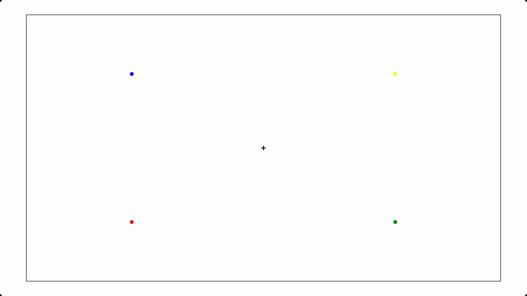
def mathView = scene.getMathView()

// Create points at key screen positions
def center = Point.at(mathView.getCenter())
    .dotStyle(DotStyle.PLUS)

def corners = [
    Point.at(mathView.getUpperLeft()),
    Point.at(mathView.getUpperRight()),
    Point.at(mathView.getLowerLeft()),
    Point.at(mathView.getLowerRight())
]

// Points at 25% and 75% positions
def Q1 = Point.at(mathView.getReltoAbsCoordinates(0.25, 0.25))
    .drawColor("red")
def Q2 = Point.at(mathView.getReltoAbsCoordinates(0.75, 0.25))
    .drawColor("green")
def Q3 = Point.at(mathView.getReltoAbsCoordinates(0.75, 0.75))
    .drawColor("yellow")
def Q4 = Point.at(mathView.getReltoAbsCoordinates(0.25, 0.75))
    .drawColor("blue")

scene.add(center, *corners, Q1, Q2, Q3, Q4)
scene.add(
    Shape.rectangle(mathView)
        .scale(0.9)  // 90% of screen size
)
Default Math View Coordinates
At initialization (16:9 aspect ratio): - Center: (0, 0) - X range: -2 to 2 - Y range: -1.125 to 1.125
Note: Y boundaries adjust automatically based on aspect ratio while maintaining the center and X boundaries.
Next Steps
Now that you understand the basic objects, explore: - Styling: Customize colors, thickness, and visual properties - Transforming Objects: Advanced positioning, scaling, and animation - Adding labels: Put names on vertices, sides and braces